


- 🍨 本文为🔗365天深度学习训练营 中的学习记录博客
- 🍖 原作者:K同学啊
一、导入库
import torch
import torch.nn as nn
import torchvision.transforms as transforms
import torchvision
from torchvision import transforms,datasets
import os,PIL,pathlib,warnings, random
from collections import OrderedDict
import torch.nn.functional as F
import torchsummary as summary
import copy
import matplotlib.pyplot as plt
查看使用的是GPU还是CPU
#忽略警告信息
warnings.filterwarnings("ignore")
#查看使用的GPU还是CPU
device = torch.device("cuda" if torch.cuda.is_available() else "cpu")
二、导入数据
#导入数据集
data_dir = './data/J3-data'
data_dir = pathlib.Path(data_dir)

data_paths  = list(data_dir.glob('*'))
#因为我的路径是data下的PotatoPlants有两级目录所以要[2]
classeNames = [str(path).split("\\")[2] for path in data_paths]
#print(classeNames) #['Early_blight', 'healthy', 'Late_blight']

#将测试集和训练集进行尺寸调整,让其符合模型想要的形式
#transforms.Compose:用于创建一个转换流水线,它接受一个转换操作的列表作为参数。
train_transforms = transforms.Compose([
    transforms.Resize([224, 224]),  # 将输入图片resize成统一尺寸
    # transforms.RandomHorizontalFlip(), # 随机水平翻转
    transforms.ToTensor(),          # 将PIL Image或numpy.ndarray转换为tensor,并归一化到[0,1]之间
    transforms.Normalize(           # 标准化处理-->转换为标准正太分布(高斯分布),使模型更容易收敛
        mean=[0.485, 0.456, 0.406],
        std=[0.229, 0.224, 0.225])  # 其中 mean=[0.485,0.456,0.406]与std=[0.229,0.224,0.225] 从数据集中随机抽样计算得到的。
])

test_transform = transforms.Compose([
    transforms.Resize([224, 224]),  # 将输入图片resize成统一尺寸
    transforms.ToTensor(),          # 将PIL Image或numpy.ndarray转换为tensor,并归一化到[0,1]之间
    transforms.Normalize(           # 标准化处理-->转换为标准正太分布(高斯分布),使模型更容易收敛
        mean=[0.485, 0.456, 0.406],
        std=[0.229, 0.224, 0.225])  # 其中 mean=[0.485,0.456,0.406]与std=[0.229,0.224,0.225] 从数据集中随机抽样计算得到的。
])

#ImageFolder:加载的图像将按照之前定义的转换流水线进行处理
total_data = datasets.ImageFolder(data_dir ,transform=train_transforms)

#划分训练集和测试集
train_size = int(0.8 * len(total_data))
test_size  = len(total_data) - train_size
train_dataset, test_dataset = torch.utils.data.random_split(total_data, [train_size, test_size])

#指定了每个批次(batch)中样本的数量,较小的batch_size可能会导致内存使用率低,但可能需要更多的迭代次数来遍历整个数据集;较大的batch_size可能会加快训练速度,但需要更多的内存。
batch_size = 32
#DataLoader:用于封装一个数据集,提供批量加载数据的功能。它使得数据的迭代更加方便,并且可以利用多线程来加速数据的加载
train_dl = torch.utils.data.DataLoader(train_dataset,
                                           batch_size=batch_size,
                                           shuffle=True,
                                           num_workers=1)
test_dl = torch.utils.data.DataLoader(test_dataset,
                                          batch_size=batch_size,
                                          shuffle=True,
                                          num_workers=1)
三、搭建模型
class DenseLayer(nn.Sequential):
    def __init__(self, in_channel, growth_rate, bn_size, drop_rate):
        super(DenseLayer, self).__init__()
        self.add_module('norm1', nn.BatchNorm2d(in_channel))
        self.add_module('relu1', nn.ReLU(inplace=True))
        self.add_module('conv1', nn.Conv2d(in_channel, bn_size*growth_rate,
                                         kernel_size=1, stride=1, bias=False))
        self.add_module('norm2', nn.BatchNorm2d(bn_size*growth_rate))
        self.add_module('relu2', nn.ReLU(inplace=True))
        self.add_module('conv2', nn.Conv2d(bn_size*growth_rate, growth_rate,
                                         kernel_size=3, stride=1, padding=1, bias=False))
        self.drop_rate = drop_rate

    def forward(self, x):
        new_feature = super(DenseLayer, self).forward(x)
        if self.drop_rate > 0:
            new_feature = F.dropout(new_feature, p=self.drop_rate, training=self.training)
        return torch.cat([x, new_feature], 1)
class DenseBlock(nn.Sequential):
    def __init__(self, num_layers, in_channel, bn_size, growth_rate, drop_rate):
        super(DenseBlock, self).__init__()
        for i in range(num_layers):
            layer = DenseLayer(in_channel + i * growth_rate, growth_rate, bn_size, drop_rate)
            self.add_module('denselayer%d' % (i + 1,), layer)
''' Transition layer between two adjacent DenseBlock '''
class Transition(nn.Sequential):
    def __init__(self, in_channel, out_channel):
        super(Transition, self).__init__()
        self.add_module('norm', nn.BatchNorm2d(in_channel))
        self.add_module('relu', nn.ReLU(inplace=True))
        self.add_module('conv', nn.Conv2d(in_channel, out_channel,
                                         kernel_size=1, stride=1, bias=False))
        self.add_module('pool', nn.AvgPool2d(2, stride=2))

class DenseNet(nn.Module):
    def __init__(self, growth_rate=32, block_config=(6,12,24,16), init_channel=64,
                 bn_size=4, compression_rate=0.5, drop_rate=0, num_classes=1000):
        '''
        :param growth_rate: (int) number of filters used in Denselayer, 'k' in the paper
        :param block_config: (list of 4 ints) number of layers in each DenseBlock
        :param init_channel: (int) number of filters in the first Conv2d
        :param bn_size: (int) the factor using in the bottleneck layer
        :param compression_rate: (float) the compression rate used in Transition Layer
        :param drop_rate: (float) the drop rate after each Denselayer
        :param num_classes: (int) 待分类的类别数
        '''
        super(DenseNet, self).__init__()
        # first Conv2d
        self.features = nn.Sequential(OrderedDict([
            ('conv0', nn.Conv2d(3, init_channel, kernel_size=7, stride=2, padding=3, bias=False)),
            ('norm0', nn.BatchNorm2d(init_channel)),
            ('relu0', nn.ReLU(inplace=True)),
            ('pool0', nn.MaxPool2d(3, stride=2, padding=1))
        ]))

        # DenseBlock
        num_features = init_channel
        for i, num_layers in enumerate(block_config):
            block = DenseBlock(num_layers, num_features, bn_size, growth_rate, drop_rate)
            self.features.add_module('denseblock%d' % (i + 1), block)
            num_features += num_layers * growth_rate
            if i != len(block_config) - 1:
                transition = Transition(num_features, int(num_features * compression_rate))
                self.features.add_module('transition%d' % (i + 1), transition)
                num_features = int(num_features * compression_rate)

        # final BN+ReLU
        self.features.add_module('norm5', nn.BatchNorm2d(num_features))
        self.features.add_module('relu5', nn.ReLU(inplace=True))

        # 分类层
        self.classifier = nn.Linear(num_features, num_classes)

        # 参数初始化
        for m in self.modules():
            if isinstance(m, nn.Conv2d):
                nn.init.kaiming_normal_(m.weight)
            elif isinstance(m, nn.BatchNorm2d):
                nn.init.constant_(m.bias, 0)
                nn.init.constant_(m.weight, 1)
            elif isinstance(m, nn.Linear):
                nn.init.constant_(m.bias, 0)

    def forward(self, x):
        x = self.features(x)
        x = F.avg_pool2d(x, 7, stride=1).view(x.size(0), -1)
        x = self.classifier(x)
        return x

device = "cuda" if torch.cuda.is_available() else "cpu"
#print("Using {} device".format(device))

densenet121 = DenseNet(init_channel=64,
                      growth_rate=32,
                      block_config=(6,12,24,16),
                      num_classes=len(classeNames))

model = densenet121.to(device)
查看参数量以及其他指标
# 统计模型参数量以及其他指标
print(summary.summary(model, (3, 224, 224)))

        Layer (type)               Output Shape         Param #
================================================================
···
     BatchNorm2d-365           [-1, 1024, 7, 7]           2,048
            ReLU-366           [-1, 1024, 7, 7]               0
          Linear-367                    [-1, 2]           2,050
================================================================
Total params: 6,955,906
Trainable params: 6,955,906
Non-trainable params: 0
----------------------------------------------------------------
Input size (MB): 0.57
Forward/backward pass size (MB): 294.57
Params size (MB): 26.53
Estimated Total Size (MB): 321.68
----------------------------------------------------------------
四、创建训练函数
def train(dataloader, model, loss_fn, optimizer):
    size = len(dataloader.dataset)  # 训练集的大小
    num_batches = len(dataloader)  # 批次数目, (size/batch_size,向上取整)

    train_loss, train_acc = 0, 0  # 初始化训练损失和正确率

    for X, y in dataloader:  # 获取图片及其标签
        X, y = X.to(device), y.to(device)

        # 计算预测误差
        pred = model(X)  # 网络输出
        loss = loss_fn(pred, y)  # 计算网络输出和真实值之间的差距,targets为真实值,计算二者差值即为损失

        # 反向传播
        optimizer.zero_grad()  # grad属性归零
        loss.backward()  # 反向传播
        optimizer.step()  # 每一步自动更新

        # 记录acc与loss
        train_acc += (pred.argmax(1) == y).type(torch.float).sum().item()
        train_loss += loss.item()

    train_acc /= size
    train_loss /= num_batches

    return train_acc, train_loss
五、创建测试函数
def test(dataloader, model, loss_fn):
    size = len(dataloader.dataset)  # 测试集的大小
    num_batches = len(dataloader)  # 批次数目, (size/batch_size,向上取整)
    test_loss, test_acc = 0, 0

    # 当不进行训练时,停止梯度更新,节省计算内存消耗
    with torch.no_grad():
        for imgs, target in dataloader:
            imgs, target = imgs.to(device), target.to(device)

            # 计算loss
            target_pred = model(imgs)
            loss = loss_fn(target_pred, target)

            test_loss += loss.item()
            test_acc += (target_pred.argmax(1) == target).type(torch.float).sum().item()

    test_acc /= size
    test_loss /= num_batches

    return test_acc, test_loss
六、主函数调用
optimizer = torch.optim.Adam(model.parameters(), lr=1e-4)
loss_fn = nn.CrossEntropyLoss()  # 创建损失函数

epochs = 20

train_loss = []
train_acc = []
test_loss = []
test_acc = []

best_acc = 0  # 设置一个最佳准确率,作为最佳模型的判别指标

if __name__ == "__main__":
    for epoch in range(epochs):

        model.train()
        epoch_train_acc, epoch_train_loss = train(train_dl, model, loss_fn, optimizer)

        model.eval()
        epoch_test_acc, epoch_test_loss = test(test_dl, model, loss_fn)

        # 保存最佳模型到 best_model
        if epoch_test_acc > best_acc:
            best_acc = epoch_test_acc
            best_model = copy.deepcopy(model)

        train_acc.append(epoch_train_acc)
        train_loss.append(epoch_train_loss)
        test_acc.append(epoch_test_acc)
        test_loss.append(epoch_test_loss)

        # 获取当前的学习率
        lr = optimizer.state_dict()['param_groups'][0]['lr']

        template = ('Epoch:{:2d}, Train_acc:{:.1f}%, Train_loss:{:.3f}, Test_acc:{:.1f}%, Test_loss:{:.3f}, Lr:{:.2E}')
        print(template.format(epoch + 1, epoch_train_acc * 100, epoch_train_loss,
                              epoch_test_acc * 100, epoch_test_loss, lr))
Epoch: 1, Train_acc:89.6%, Train_loss:0.256, Test_acc:88.4%, Test_loss:0.297, Lr:1.00E-04
Epoch: 2, Train_acc:90.4%, Train_loss:0.240, Test_acc:89.1%, Test_loss:0.268, Lr:1.00E-04
Epoch: 3, Train_acc:90.8%, Train_loss:0.223, Test_acc:87.7%, Test_loss:0.357, Lr:1.00E-04
Epoch: 4, Train_acc:91.9%, Train_loss:0.207, Test_acc:90.0%, Test_loss:0.240, Lr:1.00E-04
Epoch: 5, Train_acc:92.0%, Train_loss:0.192, Test_acc:90.3%, Test_loss:0.237, Lr:1.00E-04
Epoch: 6, Train_acc:92.8%, Train_loss:0.184, Test_acc:91.3%, Test_loss:0.210, Lr:1.00E-04
Epoch: 7, Train_acc:93.7%, Train_loss:0.161, Test_acc:89.3%, Test_loss:0.305, Lr:1.00E-04
Epoch: 8, Train_acc:94.3%, Train_loss:0.169, Test_acc:91.6%, Test_loss:0.211, Lr:1.00E-04
Epoch: 9, Train_acc:95.1%, Train_loss:0.145, Test_acc:91.3%, Test_loss:0.241, Lr:1.00E-04
Epoch:10, Train_acc:95.3%, Train_loss:0.121, Test_acc:90.2%, Test_loss:0.265, Lr:1.00E-04
Epoch:11, Train_acc:95.7%, Train_loss:0.121, Test_acc:89.9%, Test_loss:0.292, Lr:1.00E-04
Epoch:12, Train_acc:96.3%, Train_loss:0.087, Test_acc:91.2%, Test_loss:0.259, Lr:1.00E-04
Epoch:13, Train_acc:96.7%, Train_loss:0.077, Test_acc:91.7%, Test_loss:0.237, Lr:1.00E-04
Epoch:14, Train_acc:96.5%, Train_loss:0.094, Test_acc:89.2%, Test_loss:0.333, Lr:1.00E-04
Epoch:15, Train_acc:97.0%, Train_loss:0.077, Test_acc:89.5%, Test_loss:0.288, Lr:1.00E-04
Epoch:16, Train_acc:97.5%, Train_loss:0.069, Test_acc:91.5%, Test_loss:0.270, Lr:1.00E-04
Epoch:17, Train_acc:97.3%, Train_loss:0.071, Test_acc:91.3%, Test_loss:0.275, Lr:1.00E-04
Epoch:18, Train_acc:98.2%, Train_loss:0.053, Test_acc:83.9%, Test_loss:0.672, Lr:1.00E-04
Epoch:19, Train_acc:96.7%, Train_loss:0.083, Test_acc:91.9%, Test_loss:0.270, Lr:1.00E-04
Epoch:20, Train_acc:98.8%, Train_loss:0.036, Test_acc:91.0%, Test_loss:0.360, Lr:1.00E-04
最佳准确率: 0.9186870570682582

Process finished with exit code 0
保存最佳模型
# 保存最佳模型到文件中
PATH = './best_model.pth'  # 保存的参数文件名
torch.save(model.state_dict(), PATH)
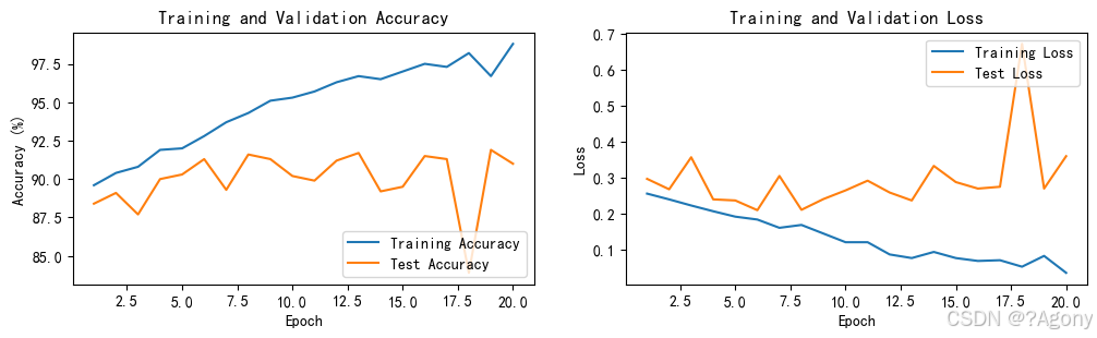
查看Loss与Accuracy图
    plt.rcParams['font.sans-serif']    = ['SimHei'] # 用来正常显示中文标签
    plt.rcParams['axes.unicode_minus'] = False      # 用来正常显示负号
    plt.rcParams['figure.dpi']         = 100        #分辨率

    epochs_range = range(epochs)

    plt.figure(figsize=(12, 3))
    plt.subplot(1, 2, 1)

    plt.plot(epochs_range, train_acc, label='Training Accuracy')
    plt.plot(epochs_range, test_acc, label='Test Accuracy')
    plt.legend(loc='lower right')
    plt.title('Training and Validation Accuracy')

    plt.subplot(1, 2, 2)
    plt.plot(epochs_range, train_loss, label='Training Loss')
    plt.plot(epochs_range, test_loss, label='Test Loss')
    plt.legend(loc='upper right')
    plt.title('Training and Validation Loss')
    plt.show()
七、小结
通过这个实例的学习,我对DenseNet算法在乳腺癌识别任务中的应用有了更深入的理解。深度学习在医学图像分析领域有着巨大的潜力,通过合理的模型设计和训练策略,我们可以更高效地解决实际问题。未来,我将继续探索更先进的算法和技术,提高在类似任务中的表现。


 1035
1035

 被折叠的 条评论
为什么被折叠?
被折叠的 条评论
为什么被折叠?
 到【灌水乐园】发言


