


- 🍨 本文为🔗365天深度学习训练营 中的学习记录博客
- 🍖 原作者:K同学啊
YOLOv5-Backbone模块实现天气预测
一、导入库
import torch
import torch.nn as nn
import torchvision.transforms as transforms
import torchvision
from torchvision import transforms, datasets
import os,PIL,pathlib,warnings
import os,PIL,random,pathlib
import torchsummary as summary
import copy
import matplotlib.pyplot as plt
#隐藏警告
import warnings
二、数据导入及分割数据集
1. 查看使用的是cpu还是gpu
warnings.filterwarnings("ignore")#忽略警告信息

device = torch.device("cuda" if torch.cuda.is_available() else "cpu")
2.导入数据及标准化
data_dir = './data/weather_photos'
data_dir = pathlib.Path(data_dir)

data_paths  = list(data_dir.glob('*'))
classeNames = [str(path).split("\\")[2] for path in data_paths]

train_transforms = transforms.Compose([
    transforms.Resize([224, 224]),  # 将输入图片resize成统一尺寸
    # transforms.RandomHorizontalFlip(), # 随机水平翻转
    transforms.ToTensor(),          # 将PIL Image或numpy.ndarray转换为tensor,并归一化到[0,1]之间
    transforms.Normalize(           # 标准化处理-->转换为标准正太分布(高斯分布),使模型更容易收敛
        mean=[0.485, 0.456, 0.406],
        std=[0.229, 0.224, 0.225])  # 其中 mean=[0.485,0.456,0.406]与std=[0.229,0.224,0.225] 从数据集中随机抽样计算得到的。
])

test_transform = transforms.Compose([
    transforms.Resize([224, 224]),  # 将输入图片resize成统一尺寸
    transforms.ToTensor(),          # 将PIL Image或numpy.ndarray转换为tensor,并归一化到[0,1]之间
    transforms.Normalize(           # 标准化处理-->转换为标准正太分布(高斯分布),使模型更容易收敛
        mean=[0.485, 0.456, 0.406],
        std=[0.229, 0.224, 0.225])  # 其中 mean=[0.485,0.456,0.406]与std=[0.229,0.224,0.225] 从数据集中随机抽样计算得到的。
])
2. 划分训练集和测试集
total_data = datasets.ImageFolder("./data/weather_photos",transform=train_transforms)
total_data# 关于transforms.Compose的更多介绍可以参考:https://blog.youkuaiyun.com/qq_38251616/article/details/124878863
train_transforms = transforms.Compose([
    transforms.Resize([224, 224]),  # 将输入图片resize成统一尺寸
    # transforms.RandomHorizontalFlip(), # 随机水平翻转
    transforms.ToTensor(),          # 将PIL Image或numpy.ndarray转换为tensor,并归一化到[0,1]之间
    transforms.Normalize(           # 标准化处理-->转换为标准正太分布(高斯分布),使模型更容易收敛
        mean=[0.485, 0.456, 0.406],
        std=[0.229, 0.224, 0.225])  # 其中 mean=[0.485,0.456,0.406]与std=[0.229,0.224,0.225] 从数据集中随机抽样计算得到的。
])

test_transform = transforms.Compose([
    transforms.Resize([224, 224]),  # 将输入图片resize成统一尺寸
    transforms.ToTensor(),          # 将PIL Image或numpy.ndarray转换为tensor,并归一化到[0,1]之间
    transforms.Normalize(           # 标准化处理-->转换为标准正太分布(高斯分布),使模型更容易收敛
        mean=[0.485, 0.456, 0.406],
        std=[0.229, 0.224, 0.225])  # 其中 mean=[0.485,0.456,0.406]与std=[0.229,0.224,0.225] 从数据集中随机抽样计算得到的。
])

total_data = datasets.ImageFolder("./data/weather_photos",transform=train_transforms)

train_size = int(0.8 * len(total_data))
test_size  = len(total_data) - train_size
train_dataset, test_dataset = torch.utils.data.random_split(total_data, [train_size, test_size])
3. 训练批次
batch_size = 4

train_dl = torch.utils.data.DataLoader(train_dataset,
                                           batch_size=batch_size,
                                           shuffle=True,
                                           num_workers=1)
test_dl = torch.utils.data.DataLoader(test_dataset,
                                          batch_size=batch_size,
                                          shuffle=True,
                                          num_workers=1)
三、搭建模型
模型结构

各模块的定义
def autopad(k, p=None):  # kernel, padding
    # Pad to 'same'
    if p is None:
        p = k // 2 if isinstance(k, int) else [x // 2 for x in k]  # auto-pad
    return p


class Conv(nn.Module):
    # Standard convolution
    def __init__(self, c1, c2, k=1, s=1, p=None, g=1, act=True):  # ch_in, ch_out, kernel, stride, padding, groups
        super().__init__()
        self.conv = nn.Conv2d(c1, c2, k, s, autopad(k, p), groups=g, bias=False)
        self.bn = nn.BatchNorm2d(c2)
        self.act = nn.SiLU() if act is True else (act if isinstance(act, nn.Module) else nn.Identity())

    def forward(self, x):
        return self.act(self.bn(self.conv(x)))


class Bottleneck(nn.Module):
    # Standard bottleneck
    def __init__(self, c1, c2, shortcut=True, g=1, e=0.5):  # ch_in, ch_out, shortcut, groups, expansion
        super().__init__()
        c_ = int(c2 * e)  # hidden channels
        self.cv1 = Conv(c1, c_, 1, 1)
        self.cv2 = Conv(c_, c2, 3, 1, g=g)
        self.add = shortcut and c1 == c2

    def forward(self, x):
        return x + self.cv2(self.cv1(x)) if self.add else self.cv2(self.cv1(x))


class C3(nn.Module):
    # CSP Bottleneck with 3 convolutions
    def __init__(self, c1, c2, n=1, shortcut=True, g=1, e=0.5):  # ch_in, ch_out, number, shortcut, groups, expansion
        super().__init__()
        c_ = int(c2 * e)  # hidden channels
        self.cv1 = Conv(c1, c_, 1, 1)
        self.cv2 = Conv(c1, c_, 1, 1)
        self.cv3 = Conv(2 * c_, c2, 1)  # act=FReLU(c2)
        self.m = nn.Sequential(*(Bottleneck(c_, c_, shortcut, g, e=1.0) for _ in range(n)))

    def forward(self, x):
        return self.cv3(torch.cat((self.m(self.cv1(x)), self.cv2(x)), dim=1))


class SPPF(nn.Module):
    # Spatial Pyramid Pooling - Fast (SPPF) layer for YOLOv5 by Glenn Jocher
    def __init__(self, c1, c2, k=5):  # equivalent to SPP(k=(5, 9, 13))
        super().__init__()
        c_ = c1 // 2  # hidden channels
        self.cv1 = Conv(c1, c_, 1, 1)
        self.cv2 = Conv(c_ * 4, c2, 1, 1)
        self.m = nn.MaxPool2d(kernel_size=k, stride=1, padding=k // 2)

    def forward(self, x):
        x = self.cv1(x)
        with warnings.catch_warnings():
            warnings.simplefilter('ignore')  # suppress torch 1.9.0 max_pool2d() warning
            y1 = self.m(x)
            y2 = self.m(y1)
            return self.cv2(torch.cat([x, y1, y2, self.m(y2)], 1))
主干网路的搭建
YOLOv5_backbone(
  (Conv_1): Conv(
    (conv): Conv2d(3, 64, kernel_size=(3, 3), stride=(2, 2), padding=(2, 2), bias=False)
    (bn): BatchNorm2d(64, eps=1e-05, momentum=0.1, affine=True, track_running_stats=True)
    (act): SiLU()
  )
  (Conv_2): Conv(
    (conv): Conv2d(64, 128, kernel_size=(3, 3), stride=(2, 2), padding=(1, 1), bias=False)
    (bn): BatchNorm2d(128, eps=1e-05, momentum=0.1, affine=True, track_running_stats=True)
    (act): SiLU()
  )
  (C3_3): C3(
    (cv1): Conv(
      (conv): Conv2d(128, 64, kernel_size=(1, 1), stride=(1, 1), bias=False)
      (bn): BatchNorm2d(64, eps=1e-05, momentum=0.1, affine=True, track_running_stats=True)
      (act): SiLU()
    )
    (cv2): Conv(
      (conv): Conv2d(128, 64, kernel_size=(1, 1), stride=(1, 1), bias=False)
      (bn): BatchNorm2d(64, eps=1e-05, momentum=0.1, affine=True, track_running_stats=True)
      (act): SiLU()
    )
    (cv3): Conv(
      (conv): Conv2d(128, 128, kernel_size=(1, 1), stride=(1, 1), bias=False)
      (bn): BatchNorm2d(128, eps=1e-05, momentum=0.1, affine=True, track_running_stats=True)
      (act): SiLU()
    )
    (m): Sequential(
      (0): Bottleneck(
        (cv1): Conv(
          (conv): Conv2d(64, 64, kernel_size=(1, 1), stride=(1, 1), bias=False)
          (bn): BatchNorm2d(64, eps=1e-05, momentum=0.1, affine=True, track_running_stats=True)
          (act): SiLU()
        )
        (cv2): Conv(
          (conv): Conv2d(64, 64, kernel_size=(3, 3), stride=(1, 1), padding=(1, 1), bias=False)
          (bn): BatchNorm2d(64, eps=1e-05, momentum=0.1, affine=True, track_running_stats=True)
          (act): SiLU()
        )
      )
    )
  )
  (Conv_4): Conv(
    (conv): Conv2d(128, 256, kernel_size=(3, 3), stride=(2, 2), padding=(1, 1), bias=False)
    (bn): BatchNorm2d(256, eps=1e-05, momentum=0.1, affine=True, track_running_stats=True)
    (act): SiLU()
  )
  (C3_5): C3(
    (cv1): Conv(
      (conv): Conv2d(256, 128, kernel_size=(1, 1), stride=(1, 1), bias=False)
      (bn): BatchNorm2d(128, eps=1e-05, momentum=0.1, affine=True, track_running_stats=True)
      (act): SiLU()
    )
    (cv2): Conv(
      (conv): Conv2d(256, 128, kernel_size=(1, 1), stride=(1, 1), bias=False)
      (bn): BatchNorm2d(128, eps=1e-05, momentum=0.1, affine=True, track_running_stats=True)
      (act): SiLU()
    )
    (cv3): Conv(
      (conv): Conv2d(256, 256, kernel_size=(1, 1), stride=(1, 1), bias=False)
      (bn): BatchNorm2d(256, eps=1e-05, momentum=0.1, affine=True, track_running_stats=True)
      (act): SiLU()
    )
    (m): Sequential(
      (0): Bottleneck(
        (cv1): Conv(
          (conv): Conv2d(128, 128, kernel_size=(1, 1), stride=(1, 1), bias=False)
          (bn): BatchNorm2d(128, eps=1e-05, momentum=0.1, affine=True, track_running_stats=True)
          (act): SiLU()
        )
        (cv2): Conv(
          (conv): Conv2d(128, 128, kernel_size=(3, 3), stride=(1, 1), padding=(1, 1), bias=False)
          (bn): BatchNorm2d(128, eps=1e-05, momentum=0.1, affine=True, track_running_stats=True)
          (act): SiLU()
        )
      )
    )
  )
  (Conv_6): Conv(
    (conv): Conv2d(256, 512, kernel_size=(3, 3), stride=(2, 2), padding=(1, 1), bias=False)
    (bn): BatchNorm2d(512, eps=1e-05, momentum=0.1, affine=True, track_running_stats=True)
    (act): SiLU()
  )
  (C3_7): C3(
    (cv1): Conv(
      (conv): Conv2d(512, 256, kernel_size=(1, 1), stride=(1, 1), bias=False)
      (bn): BatchNorm2d(256, eps=1e-05, momentum=0.1, affine=True, track_running_stats=True)
      (act): SiLU()
    )
    (cv2): Conv(
      (conv): Conv2d(512, 256, kernel_size=(1, 1), stride=(1, 1), bias=False)
      (bn): BatchNorm2d(256, eps=1e-05, momentum=0.1, affine=True, track_running_stats=True)
      (act): SiLU()
    )
    (cv3): Conv(
      (conv): Conv2d(512, 512, kernel_size=(1, 1), stride=(1, 1), bias=False)
      (bn): BatchNorm2d(512, eps=1e-05, momentum=0.1, affine=True, track_running_stats=True)
      (act): SiLU()
    )
    (m): Sequential(
      (0): Bottleneck(
        (cv1): Conv(
          (conv): Conv2d(256, 256, kernel_size=(1, 1), stride=(1, 1), bias=False)
          (bn): BatchNorm2d(256, eps=1e-05, momentum=0.1, affine=True, track_running_stats=True)
          (act): SiLU()
        )
        (cv2): Conv(
          (conv): Conv2d(256, 256, kernel_size=(3, 3), stride=(1, 1), padding=(1, 1), bias=False)
          (bn): BatchNorm2d(256, eps=1e-05, momentum=0.1, affine=True, track_running_stats=True)
          (act): SiLU()
        )
      )
    )
  )
  (Conv_8): Conv(
    (conv): Conv2d(512, 1024, kernel_size=(3, 3), stride=(2, 2), padding=(1, 1), bias=False)
    (bn): BatchNorm2d(1024, eps=1e-05, momentum=0.1, affine=True, track_running_stats=True)
    (act): SiLU()
  )
  (C3_9): C3(
    (cv1): Conv(
      (conv): Conv2d(1024, 512, kernel_size=(1, 1), stride=(1, 1), bias=False)
      (bn): BatchNorm2d(512, eps=1e-05, momentum=0.1, affine=True, track_running_stats=True)
      (act): SiLU()
    )
    (cv2): Conv(
      (conv): Conv2d(1024, 512, kernel_size=(1, 1), stride=(1, 1), bias=False)
      (bn): BatchNorm2d(512, eps=1e-05, momentum=0.1, affine=True, track_running_stats=True)
      (act): SiLU()
    )
    (cv3): Conv(
      (conv): Conv2d(1024, 1024, kernel_size=(1, 1), stride=(1, 1), bias=False)
      (bn): BatchNorm2d(1024, eps=1e-05, momentum=0.1, affine=True, track_running_stats=True)
      (act): SiLU()
    )
    (m): Sequential(
      (0): Bottleneck(
        (cv1): Conv(
          (conv): Conv2d(512, 512, kernel_size=(1, 1), stride=(1, 1), bias=False)
          (bn): BatchNorm2d(512, eps=1e-05, momentum=0.1, affine=True, track_running_stats=True)
          (act): SiLU()
        )
        (cv2): Conv(
          (conv): Conv2d(512, 512, kernel_size=(3, 3), stride=(1, 1), padding=(1, 1), bias=False)
          (bn): BatchNorm2d(512, eps=1e-05, momentum=0.1, affine=True, track_running_stats=True)
          (act): SiLU()
        )
      )
    )
  )
  (SPPF): SPPF(
    (cv1): Conv(
      (conv): Conv2d(1024, 512, kernel_size=(1, 1), stride=(1, 1), bias=False)
      (bn): BatchNorm2d(512, eps=1e-05, momentum=0.1, affine=True, track_running_stats=True)
      (act): SiLU()
    )
    (cv2): Conv(
      (conv): Conv2d(2048, 1024, kernel_size=(1, 1), stride=(1, 1), bias=False)
      (bn): BatchNorm2d(1024, eps=1e-05, momentum=0.1, affine=True, track_running_stats=True)
      (act): SiLU()
    )
    (m): MaxPool2d(kernel_size=5, stride=1, padding=2, dilation=1, ceil_mode=False)
  )
  (classifier): Sequential(
    (0): Linear(in_features=65536, out_features=100, bias=True)
    (1): ReLU()
    (2): Linear(in_features=100, out_features=4, bias=True)
  )
)

Process finished with exit code -1
查看模型详情
#print(summary.summary(model, (3, 224, 224)))
----------------------------------------------------------------
        Layer (type)               Output Shape         Param #
================================================================
            Conv2d-1         [-1, 64, 113, 113]           1,728
       BatchNorm2d-2         [-1, 64, 113, 113]             128
              SiLU-3         [-1, 64, 113, 113]               0
              Conv-4         [-1, 64, 113, 113]               0
            Conv2d-5          [-1, 128, 57, 57]          73,728
       BatchNorm2d-6          [-1, 128, 57, 57]             256
              SiLU-7          [-1, 128, 57, 57]               0
              Conv-8          [-1, 128, 57, 57]               0
            Conv2d-9           [-1, 64, 57, 57]           8,192
      BatchNorm2d-10           [-1, 64, 57, 57]             128
             SiLU-11           [-1, 64, 57, 57]               0
             Conv-12           [-1, 64, 57, 57]               0
           Conv2d-13           [-1, 64, 57, 57]           4,096
      BatchNorm2d-14           [-1, 64, 57, 57]             128
             SiLU-15           [-1, 64, 57, 57]               0
             Conv-16           [-1, 64, 57, 57]               0
           Conv2d-17           [-1, 64, 57, 57]          36,864
      BatchNorm2d-18           [-1, 64, 57, 57]             128
             SiLU-19           [-1, 64, 57, 57]               0
             Conv-20           [-1, 64, 57, 57]               0
       Bottleneck-21           [-1, 64, 57, 57]               0
           Conv2d-22           [-1, 64, 57, 57]           8,192
      BatchNorm2d-23           [-1, 64, 57, 57]             128
             SiLU-24           [-1, 64, 57, 57]               0
             Conv-25           [-1, 64, 57, 57]               0
           Conv2d-26          [-1, 128, 57, 57]          16,384
      BatchNorm2d-27          [-1, 128, 57, 57]             256
             SiLU-28          [-1, 128, 57, 57]               0
             Conv-29          [-1, 128, 57, 57]               0
               C3-30          [-1, 128, 57, 57]               0
           Conv2d-31          [-1, 256, 29, 29]         294,912
      BatchNorm2d-32          [-1, 256, 29, 29]             512
             SiLU-33          [-1, 256, 29, 29]               0
             Conv-34          [-1, 256, 29, 29]               0
           Conv2d-35          [-1, 128, 29, 29]          32,768
      BatchNorm2d-36          [-1, 128, 29, 29]             256
             SiLU-37          [-1, 128, 29, 29]               0
             Conv-38          [-1, 128, 29, 29]               0
           Conv2d-39          [-1, 128, 29, 29]          16,384
      BatchNorm2d-40          [-1, 128, 29, 29]             256
             SiLU-41          [-1, 128, 29, 29]               0
             Conv-42          [-1, 128, 29, 29]               0
           Conv2d-43          [-1, 128, 29, 29]         147,456
      BatchNorm2d-44          [-1, 128, 29, 29]             256
             SiLU-45          [-1, 128, 29, 29]               0
             Conv-46          [-1, 128, 29, 29]               0
       Bottleneck-47          [-1, 128, 29, 29]               0
           Conv2d-48          [-1, 128, 29, 29]          32,768
      BatchNorm2d-49          [-1, 128, 29, 29]             256
             SiLU-50          [-1, 128, 29, 29]               0
             Conv-51          [-1, 128, 29, 29]               0
           Conv2d-52          [-1, 256, 29, 29]          65,536
      BatchNorm2d-53          [-1, 256, 29, 29]             512
             SiLU-54          [-1, 256, 29, 29]               0
             Conv-55          [-1, 256, 29, 29]               0
               C3-56          [-1, 256, 29, 29]               0
           Conv2d-57          [-1, 512, 15, 15]       1,179,648
      BatchNorm2d-58          [-1, 512, 15, 15]           1,024
             SiLU-59          [-1, 512, 15, 15]               0
             Conv-60          [-1, 512, 15, 15]               0
           Conv2d-61          [-1, 256, 15, 15]         131,072
      BatchNorm2d-62          [-1, 256, 15, 15]             512
             SiLU-63          [-1, 256, 15, 15]               0
             Conv-64          [-1, 256, 15, 15]               0
           Conv2d-65          [-1, 256, 15, 15]          65,536
      BatchNorm2d-66          [-1, 256, 15, 15]             512
             SiLU-67          [-1, 256, 15, 15]               0
             Conv-68          [-1, 256, 15, 15]               0
           Conv2d-69          [-1, 256, 15, 15]         589,824
      BatchNorm2d-70          [-1, 256, 15, 15]             512
             SiLU-71          [-1, 256, 15, 15]               0
             Conv-72          [-1, 256, 15, 15]               0
       Bottleneck-73          [-1, 256, 15, 15]               0
           Conv2d-74          [-1, 256, 15, 15]         131,072
      BatchNorm2d-75          [-1, 256, 15, 15]             512
             SiLU-76          [-1, 256, 15, 15]               0
             Conv-77          [-1, 256, 15, 15]               0
           Conv2d-78          [-1, 512, 15, 15]         262,144
      BatchNorm2d-79          [-1, 512, 15, 15]           1,024
             SiLU-80          [-1, 512, 15, 15]               0
             Conv-81          [-1, 512, 15, 15]               0
               C3-82          [-1, 512, 15, 15]               0
           Conv2d-83           [-1, 1024, 8, 8]       4,718,592
      BatchNorm2d-84           [-1, 1024, 8, 8]           2,048
             SiLU-85           [-1, 1024, 8, 8]               0
             Conv-86           [-1, 1024, 8, 8]               0
           Conv2d-87            [-1, 512, 8, 8]         524,288
      BatchNorm2d-88            [-1, 512, 8, 8]           1,024
             SiLU-89            [-1, 512, 8, 8]               0
             Conv-90            [-1, 512, 8, 8]               0
           Conv2d-91            [-1, 512, 8, 8]         262,144
      BatchNorm2d-92            [-1, 512, 8, 8]           1,024
             SiLU-93            [-1, 512, 8, 8]               0
             Conv-94            [-1, 512, 8, 8]               0
           Conv2d-95            [-1, 512, 8, 8]       2,359,296
      BatchNorm2d-96            [-1, 512, 8, 8]           1,024
             SiLU-97            [-1, 512, 8, 8]               0
             Conv-98            [-1, 512, 8, 8]               0
       Bottleneck-99            [-1, 512, 8, 8]               0
          Conv2d-100            [-1, 512, 8, 8]         524,288
     BatchNorm2d-101            [-1, 512, 8, 8]           1,024
            SiLU-102            [-1, 512, 8, 8]               0
            Conv-103            [-1, 512, 8, 8]               0
          Conv2d-104           [-1, 1024, 8, 8]       1,048,576
     BatchNorm2d-105           [-1, 1024, 8, 8]           2,048
            SiLU-106           [-1, 1024, 8, 8]               0
            Conv-107           [-1, 1024, 8, 8]               0
              C3-108           [-1, 1024, 8, 8]               0
          Conv2d-109            [-1, 512, 8, 8]         524,288
     BatchNorm2d-110            [-1, 512, 8, 8]           1,024
            SiLU-111            [-1, 512, 8, 8]               0
            Conv-112            [-1, 512, 8, 8]               0
       MaxPool2d-113            [-1, 512, 8, 8]               0
       MaxPool2d-114            [-1, 512, 8, 8]               0
       MaxPool2d-115            [-1, 512, 8, 8]               0
          Conv2d-116           [-1, 1024, 8, 8]       2,097,152
     BatchNorm2d-117           [-1, 1024, 8, 8]           2,048
            SiLU-118           [-1, 1024, 8, 8]               0
            Conv-119           [-1, 1024, 8, 8]               0
            SPPF-120           [-1, 1024, 8, 8]               0
          Linear-121                  [-1, 100]       6,553,700
            ReLU-122                  [-1, 100]               0
          Linear-123                    [-1, 4]             404
================================================================
Total params: 21,729,592
Trainable params: 21,729,592
Non-trainable params: 0
----------------------------------------------------------------
Input size (MB): 0.57
Forward/backward pass size (MB): 137.59
Params size (MB): 82.89
Estimated Total Size (MB): 221.06
----------------------------------------------------------------

Process finished with exit code 0
四、训练函数
# 训练循环
def train(dataloader, model, loss_fn, optimizer):
    size = len(dataloader.dataset)  # 训练集的大小
    num_batches = len(dataloader)  # 批次数目, (size/batch_size,向上取整)

    train_loss, train_acc = 0, 0  # 初始化训练损失和正确率

    for X, y in dataloader:  # 获取图片及其标签
        X, y = X.to(device), y.to(device)

        # 计算预测误差
        pred = model(X)  # 网络输出
        loss = loss_fn(pred, y)  # 计算网络输出和真实值之间的差距,targets为真实值,计算二者差值即为损失

        # 反向传播
        optimizer.zero_grad()  # grad属性归零
        loss.backward()  # 反向传播
        optimizer.step()  # 每一步自动更新

        # 记录acc与loss
        train_acc += (pred.argmax(1) == y).type(torch.float).sum().item()
        train_loss += loss.item()

    train_acc /= size
    train_loss /= num_batches

    return train_acc, train_loss
五、测试函数
def test(dataloader, model, loss_fn):
    size = len(dataloader.dataset)  # 测试集的大小
    num_batches = len(dataloader)  # 批次数目, (size/batch_size,向上取整)
    test_loss, test_acc = 0, 0

    # 当不进行训练时,停止梯度更新,节省计算内存消耗
    with torch.no_grad():
        for imgs, target in dataloader:
            imgs, target = imgs.to(device), target.to(device)

            # 计算loss
            target_pred = model(imgs)
            loss = loss_fn(target_pred, target)

            test_loss += loss.item()
            test_acc += (target_pred.argmax(1) == target).type(torch.float).sum().item()

    test_acc /= size
    test_loss /= num_batches

    return test_acc, test_loss
五、正式训练
optimizer = torch.optim.Adam(model.parameters(), lr=1e-4)
loss_fn = nn.CrossEntropyLoss()  # 创建损失函数

epochs = 30

train_loss = []
train_acc = []
test_loss = []
test_acc = []

best_acc = 0  # 设置一个最佳准确率,作为最佳模型的判别指标

if __name__ == '__main__':
    for epoch in range(epochs):

        model.train()
        epoch_train_acc, epoch_train_loss = train(train_dl, model, loss_fn, optimizer)

        model.eval()
        epoch_test_acc, epoch_test_loss = test(test_dl, model, loss_fn)

        # 保存最佳模型到 best_model
        if epoch_test_acc > best_acc:
            best_acc = epoch_test_acc
            best_model = copy.deepcopy(model)

        train_acc.append(epoch_train_acc)
        train_loss.append(epoch_train_loss)
        test_acc.append(epoch_test_acc)
        test_loss.append(epoch_test_loss)

        # 获取当前的学习率
        lr = optimizer.state_dict()['param_groups'][0]['lr']

        template = ('Epoch:{:2d}, Train_acc:{:.1f}%, Train_loss:{:.3f}, Test_acc:{:.1f}%, Test_loss:{:.3f}, Lr:{:.2E}')
        print(template.format(epoch + 1, epoch_train_acc * 100, epoch_train_loss,
                              epoch_test_acc * 100, epoch_test_loss, lr))
六、保存最佳模型
    # 保存最佳模型到文件中
    PATH = './best_model.pth'  # 保存的参数文件名
    torch.save(model.state_dict(), PATH)
模型调用
参考之前几周的模型调用方法即可,本篇不做过多的赘述了
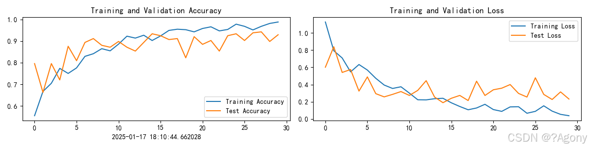
七、可视化测试过程准确率和损失值的可视化过程
warnings.filterwarnings("ignore")               #忽略警告信息
    plt.rcParams['font.sans-serif']    = ['SimHei'] # 用来正常显示中文标签
    plt.rcParams['axes.unicode_minus'] = False      # 用来正常显示负号
    plt.rcParams['figure.dpi']         = 100        #分辨率

    epochs_range = range(epochs)

    plt.figure(figsize=(12, 3))
    plt.subplot(1, 2, 1)

    plt.plot(epochs_range, train_acc, label='Training Accuracy')
    plt.plot(epochs_range, test_acc, label='Test Accuracy')
    plt.legend(loc='lower right')
    plt.title('Training and Validation Accuracy')

    plt.subplot(1, 2, 2)
    plt.plot(epochs_range, train_loss, label='Training Loss')
    plt.plot(epochs_range, test_loss, label='Test Loss')
    plt.legend(loc='upper right')
    plt.title('Training and Validation Loss')
    plt.show()
Epoch: 1, Train_acc:55.4%, Train_loss:1.127, Test_acc:79.6%, Test_loss:0.602, Lr:1.00E-04
Epoch: 2, Train_acc:66.7%, Train_loss:0.793, Test_acc:66.2%, Test_loss:0.840, Lr:1.00E-04
Epoch: 3, Train_acc:70.4%, Train_loss:0.709, Test_acc:79.6%, Test_loss:0.541, Lr:1.00E-04
Epoch: 4, Train_acc:77.3%, Train_loss:0.547, Test_acc:72.0%, Test_loss:0.575, Lr:1.00E-04
Epoch: 5, Train_acc:75.0%, Train_loss:0.633, Test_acc:87.6%, Test_loss:0.324, Lr:1.00E-04
Epoch: 6, Train_acc:77.6%, Train_loss:0.569, Test_acc:80.9%, Test_loss:0.489, Lr:1.00E-04
Epoch: 7, Train_acc:82.9%, Train_loss:0.473, Test_acc:89.3%, Test_loss:0.294, Lr:1.00E-04
Epoch: 8, Train_acc:84.1%, Train_loss:0.395, Test_acc:91.1%, Test_loss:0.257, Lr:1.00E-04
Epoch: 9, Train_acc:86.4%, Train_loss:0.355, Test_acc:88.0%, Test_loss:0.286, Lr:1.00E-04
Epoch:10, Train_acc:85.4%, Train_loss:0.374, Test_acc:87.1%, Test_loss:0.319, Lr:1.00E-04
Epoch:11, Train_acc:88.6%, Train_loss:0.300, Test_acc:89.8%, Test_loss:0.274, Lr:1.00E-04
Epoch:12, Train_acc:92.2%, Train_loss:0.223, Test_acc:87.1%, Test_loss:0.332, Lr:1.00E-04
Epoch:13, Train_acc:91.3%, Train_loss:0.222, Test_acc:85.3%, Test_loss:0.445, Lr:1.00E-04
Epoch:14, Train_acc:92.7%, Train_loss:0.236, Test_acc:89.3%, Test_loss:0.255, Lr:1.00E-04
Epoch:15, Train_acc:90.2%, Train_loss:0.240, Test_acc:93.3%, Test_loss:0.189, Lr:1.00E-04
Epoch:16, Train_acc:92.3%, Train_loss:0.188, Test_acc:92.4%, Test_loss:0.241, Lr:1.00E-04
Epoch:17, Train_acc:94.9%, Train_loss:0.145, Test_acc:90.7%, Test_loss:0.274, Lr:1.00E-04
Epoch:18, Train_acc:95.4%, Train_loss:0.107, Test_acc:91.1%, Test_loss:0.214, Lr:1.00E-04
Epoch:19, Train_acc:95.2%, Train_loss:0.128, Test_acc:82.2%, Test_loss:0.439, Lr:1.00E-04
Epoch:20, Train_acc:94.2%, Train_loss:0.170, Test_acc:92.0%, Test_loss:0.273, Lr:1.00E-04
Epoch:21, Train_acc:95.8%, Train_loss:0.109, Test_acc:88.4%, Test_loss:0.339, Lr:1.00E-04
Epoch:22, Train_acc:96.6%, Train_loss:0.088, Test_acc:90.2%, Test_loss:0.358, Lr:1.00E-04
Epoch:23, Train_acc:94.7%, Train_loss:0.140, Test_acc:85.3%, Test_loss:0.400, Lr:1.00E-04
Epoch:24, Train_acc:95.3%, Train_loss:0.142, Test_acc:92.4%, Test_loss:0.297, Lr:1.00E-04
Epoch:25, Train_acc:97.8%, Train_loss:0.066, Test_acc:93.3%, Test_loss:0.255, Lr:1.00E-04
Epoch:26, Train_acc:96.8%, Train_loss:0.089, Test_acc:90.2%, Test_loss:0.479, Lr:1.00E-04
Epoch:27, Train_acc:95.1%, Train_loss:0.153, Test_acc:93.8%, Test_loss:0.286, Lr:1.00E-04
Epoch:28, Train_acc:96.8%, Train_loss:0.091, Test_acc:94.2%, Test_loss:0.226, Lr:1.00E-04
Epoch:29, Train_acc:98.1%, Train_loss:0.054, Test_acc:89.8%, Test_loss:0.315, Lr:1.00E-04
Epoch:30, Train_acc:98.8%, Train_loss:0.038, Test_acc:92.9%, Test_loss:0.232, Lr:1.00E-04
Done

Process finished with exit code 0


Process finished with exit code 0
总结
- 概述
- YOLOv5的Backbone(骨干网络)模块是YOLOv5架构中的关键部分。它的主要作用是提取图像的特征,为后续的目标检测任务提供丰富的语义信息。
- 具体网络结构及功能
- CSPNet(Cross Stage Partial Network)结构:
- YOLOv5 - Backbone部分采用了CSPNet结构。CSPNet的核心思想是通过跨阶段的局部连接,减少计算量的同时增强网络的学习能力。例如,它将基础层的特征映射分成两部分,一部分经过一系列卷积层等操作,另一部分直接与前面操作后的结果进行拼接。这样可以有效防止梯度消失问题,使得网络能够更好地训练深层网络。
- Focus结构:
- Focus模块是YOLOv5 Backbone的一个创新点。它的主要作用是进行切片操作,在输入图像进入网络的初期,对图像进行下采样。具体来说,它将一张输入图像的每个通道,按照一定规则进行切片,比如将一个(W\times H)大小的通道切片为(W/2\times H/2)大小的4个切片,然后将这些切片在通道维度上进行拼接。这样做的好处是可以在不丢失太多信息的情况下,增加通道数,提高特征提取的效率。
- 卷积层(Convolution Layers):
- 包含多个卷积层,这些卷积层用于提取图像的不同层次的特征。通常卷积核大小有(3\times3)等。通过不断地卷积操作,网络可以逐步提取从低级的边缘、纹理等特征到高级的物体形状、类别等语义特征。例如,在网络的浅层部分,卷积层可以提取图像中的边缘和简单纹理信息;随着网络的深入,通过多次卷积和池化等操作的组合,能够提取出更复杂的物体特征,如物体的整体轮廓和类别相关的特征。
- CSPNet(Cross Stage Partial Network)结构:
- 在目标检测中的重要性
- 高质量的特征提取是准确目标检测的基础。Backbone模块提取的特征能够帮助后续的检测头(Detection Head)确定目标的位置、类别等信息。如果Backbone模块提取的特征不够准确或者丰富,那么检测头就很难准确地判断目标的位置和类别,从而影响整个目标检测系统的性能。例如,在检测复杂场景中的小目标时,一个好的Backbone模块能够提取到足够精细的特征,使得检测头能够准确地定位和识别这些小目标。


 1110
1110

 被折叠的 条评论
为什么被折叠?
被折叠的 条评论
为什么被折叠?
 到【灌水乐园】发言


