


 本文深入探讨了LightGBM的工作原理及其关键优化技术GOSS和EFB,详细解释了梯度下降、提升和GBDT的基本概念,以及如何通过采样和特征捆绑减少计算复杂度。
墙外的一篇文章,讲得挺好的,转过来了,原文
Understanding GOSS and EFB; The core pillars of LightGBM
The post is structured as follows :
- Basics of GBM.
- Computational bottlenecks of GBM.
- LightGBM’s optimisations over these bottlenecks
Basics of GBM — Gradient Descent, Boosting and GBDT.
What is Gradient Descent?
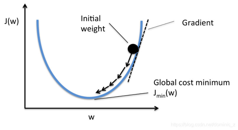
It is an optimisation technique to reduce the loss function by following the slope through a fixed step size.
What is a Boosting?
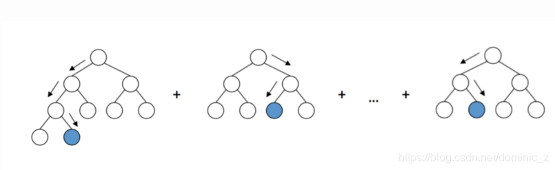
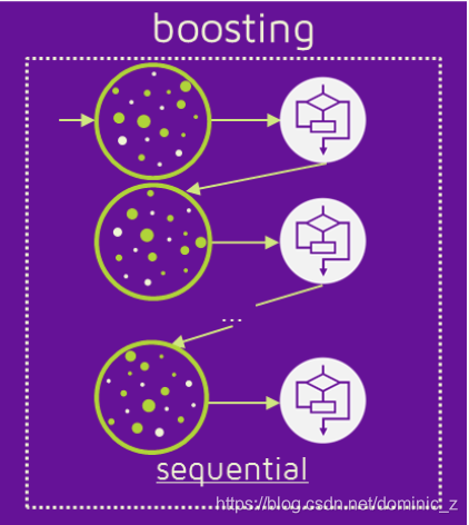
Boosting is sequential ensembling technique where hard to classify instances are given more weights. This essentially means subsequent learners would put more emphasis on learning mis-classified data instances. Final model would be weighted average of n weak learners.
Subsequent learners give more emphasis on undertrained / wrongly classified samples. Variation in dot size is representative of the weights given to that instance. Larger the size of dot larger is the weight assigned to it. Do note that all models are sequential.
What is GBDT?
GBDT (Gradient Boosting Decision Tree) is an ensemble model of decision trees which are trained in sequence(i.e. an ensemble model of boosting). In each iteration GBDT learns the decision tree by fitting the residual errors (errors upto the current iteration). This means every subsequent learner tries to learn the difference between actual output and weighted sum of predictions until an iteration before. The errors are minimised using the gradient method.
This brings us to second part of the post. The costliest operation in GBDT is training the decision tree and the most time consuming task is to find the optimum split points.
What are split points?
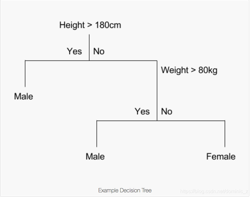
Split points are the feature values depending on which data is divided at a tree node. In the above example data division happens at node1 on Height ( 180 ) and at node 2 on Weight ( 80 ). The optimum splits are selected from a pool of candidate splits on the basis of information gain. In other words split points with maximum information gain are selected.
How are the optimum split points created?
Split finding algorithms are used to find candidate splits.
One of the most popular split finding algorithm is the Pre-sorted algorithm which enumerates all possible split points on pre-sorted values. This method is simple but highly inefficient in terms of computation power and memory .
The second method is the Histogram based algorithm which buckets continuous features into discrete bins to construct feature histograms during training. It costs O(#data * #feature) for histogram building and O(#bin * #feature) for split point finding. As bin << data histogram building will dominate the computational complexity.
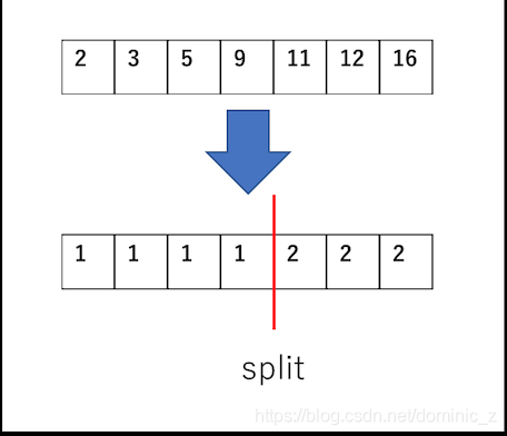
(Binning example : Binning has greatly reduced the number of candidate splits)
Both LightGBM and xgboost utilise histogram based split finding in contrast to sklearn which uses GBM ( One of the reasons why it is slow). Let’s begin with the crux of this post
What makes LightGBM special?
LightGBM aims to reduce complexity of histogram building ( O(data * feature) ) by down sampling data and feature using GOSS and EFB. This will bring down the complexity to (O(data2 * bundles)) where data2 < data and bundles << feature.
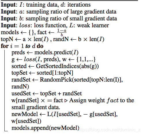
What is GOSS?
GOSS (Gradient Based One Side Sampling) is a novel sampling method which down samples the instances on basis of gradients. As we know instances with small gradients are well trained (small training error) and those with large gradients are under trained. A naive approach to downsample is to discard instances with small gradients by solely focussing on instances with large gradients but this would alter the data distribution. In a nutshell GOSS retains instances with large gradients while performing random sampling on instances with small gradients.
- Intuitive steps for GOSS calculation
- Sort the instances according to absolute gradients in a descending order
- Select the top a * 100% instances. [ Under trained / large gradients ]
- Randomly samples b * 100% instances from the rest of the data. This will reduce the contribution of well trained examples by a factor of b ( b < 1 )
- Without point 3 count of samples having small gradients would be 1-a ( currently it is b ). In order to maintain the original distribution LightGBM amplifies the contribution of samples having small gradients by a constant (1-a)/b to put more focus on the under-trained instances. This puts more focus on the under trained instances without changing the data distribution by much.
- Formal algorithm for GOSS
What is EFB(Exclusive Feature Bundling)?
Remember histogram building takes O(#data * #feature). If we are able to down sample the #feature we will speed up tree learning. LightGBM achieves this by bundling features together. We generally work with high dimensionality data. Such data have many features which are mutually exclusive i.e they never take zero values simultaneously. LightGBM safely identifies such features and bundles them into a single feature to reduce the complexity to O(#data * #bundle) where #bundle << #feature.
- Part 1 of EFB : Identifying features that could be bundled together
Intuitive explanation for creating feature bundles
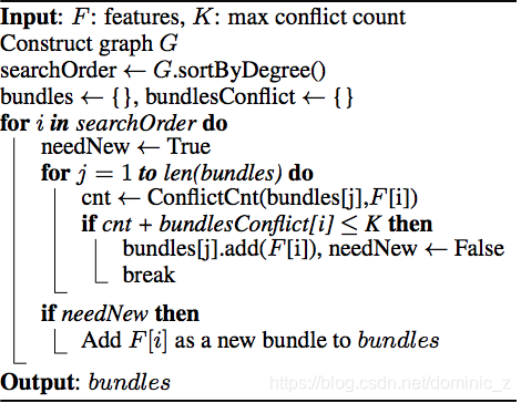
- Construct a graph with weighted (measure of conflict between features) edges. Conflict is measure of the fraction of exclusive features which have overlapping non zero values.
- Sort the features by count of non zero instances in descending order.
- Loop over the ordered list of features and assign the feature to an existing bundle (if conflict < threshold) or create a new bundle (if conflict > threshold).
Formal algorithm for bundling features
What is EFB achieving?
EFB is merging the features to reduce the training complexity. In order to keep the merge reversible we will keep exclusive features reside in different bins.
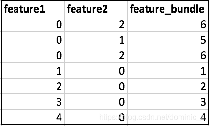
Example of the merge
In the example below you can see that feature1 and feature2 are mutually exclusive. In order to achieve non overlapping buckets we add bundle size of feature1 to feature2. This makes sure that non zero data points of bundled features ( feature1 and feature2 ) reside in different buckets. In feature_bundle buckets 1 to 4 contains non zero instances of feature1 and buckets 5,6 contain non zero instances of feature2.
(Intuitive explanation for merging features)
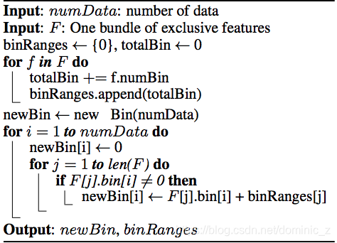
- Calculate the offset to be added to every feature in feature bundle.
- Iterate over every data instance and feature.
- Initialise the new bucket as zero for instances where all features are zero.
- Calculate the new bucket for every non zero instance of a feature by adding respective offset to original bucket of that feature.
博主注:其实我一直搞不清楚的就是这块,究竟是怎么把bundle里的特征merge到一起的,结合上面的例子来看下面的算法,bin就是一个桶,比如说一个特征的取值范围是(0,20),假如分两个bin,那就是0到10第一个bin,10到20第二个bin。又例如上面的例子,feature1的binRange就是4,feature2的binRange就是2。于是经过第一个for之后,binRanges就是{0,4,6},totalBin就是6。newBin,就是merge之后的特征的取值范围,以上面为例,返回的就是{1,2,3,4,5,6}。
Formal Algorithm for merging features
With this we have covered most of the optimisations proposed in the original paper. I hope this post would give you gain some understanding behind the core concepts of LightGBM library.
With this I complete my first attempt at writing a blog. Please feel free to share your thoughts, feedback or suggestions below.


 1156
1156

 被折叠的 条评论
为什么被折叠?
被折叠的 条评论
为什么被折叠?
 到【灌水乐园】发言


