SHAP分析完全指南：解锁机器学习模型的黑盒秘密

最新推荐文章于 2025-10-07 20:04:46 发布

原创最新推荐文章于 2025-10-07 20:04:46 发布 · 1.6k 阅读

13 ·

CC 4.0 BY-SA版权

文章标签：

#机器学习 #人工智能 #SHAP分析完全指南 #解锁机器学习模型的黑盒秘密

该文章已生成可运行项目，

摘要

在机器学习和深度学习日益普及的今天，模型的可解释性变得越来越重要。SHAP（SHapley Additive exPlanations）作为一种基于博弈论的模型解释工具，能够帮助我们理解复杂模型的决策过程，量化每个特征对预测结果的贡献。本文将深入探讨SHAP在多目标变量场景下的应用，包括多输出回归和多分类任务。通过丰富的实践示例、详细的代码演示和可视化图表，帮助读者快速掌握SHAP分析的核心概念和实际应用。文章还将涵盖注意事项、最佳实践建议以及常见问题解答，确保读者能够高效应用所学知识，提升模型的可解释性和可信度。

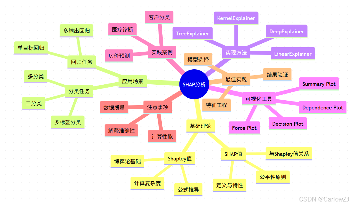
思维导图：SHAP分析知识点全景

在这里插入图片描述

mindmap
  root((SHAP分析))
    基础理论
      Shapley值
        博弈论基础
        公式推导
        计算复杂度
      SHAP值
        定义与特性
        与Shapley值关系
        公平性原则
    应用场景
      回归任务
        单目标回归
        多输出回归
      分类任务
        二分类
        多分类
        多标签分类
    实现方法
      TreeExplainer
      LinearExplainer
      KernelExplainer
      DeepExplainer
    可视化工具
      Summary Plot
      Force Plot
      Decision Plot
      Dependence Plot
    实践案例
      房价预测
      客户分类
      医疗诊断
    注意事项
      计算性能
      解释准确性
      数据质量
    最佳实践
      模型选择
      特征工程
      结果验证

1. SHAP基础理论

1.1 SHAP值的概念

SHAP（SHapley Additive exPlanations）是一种统一的框架，用于解释任何机器学习模型的输出。它基于博弈论中的Shapley值概念，能够为每个特征分配一个值来表示该特征对模型预测的贡献。

SHAP值具有以下重要特性：

公平性：所有特征的SHAP值之和等于模型的输出与基准值（通常是训练集的平均预测值）之差
局部解释性：可以解释单个预测结果
全局解释性：可以通过聚合SHAP值来解释整个数据集
一致性：如果一个模型在某个特征上变化更大，则该特征应具有更高的SHAP值

1.2 Shapley值的数学原理

Shapley值来源于合作博弈论，用于公平分配合作博弈中产生的收益。在机器学习的上下文中，我们可以将每个特征视为一个"玩家"，模型预测作为"收益"。

Shapley值的计算公式如下：

$\phi_i = \sum_{S \subseteq F \setminus \{i\}} \frac{|S|!(|F|-|S|-1)!}{|F|!} [f(S \cup \{i\}) - f(S)]$

其中：

$\phi_i$ 是特征 $i$ 的SHAP值
$S$ 是不包含特征 $i$ 的特征子集
$F$ 是所有特征的集合
$f (S)$ 是模型在特征子集 $S$ 上的输出

这个公式计算了特征 $i$ 在所有可能的特征组合中的边际贡献的加权平均。

1.3 SHAP值的计算方法

由于Shapley值的精确计算复杂度是指数级的，SHAP提供了多种近似计算方法：

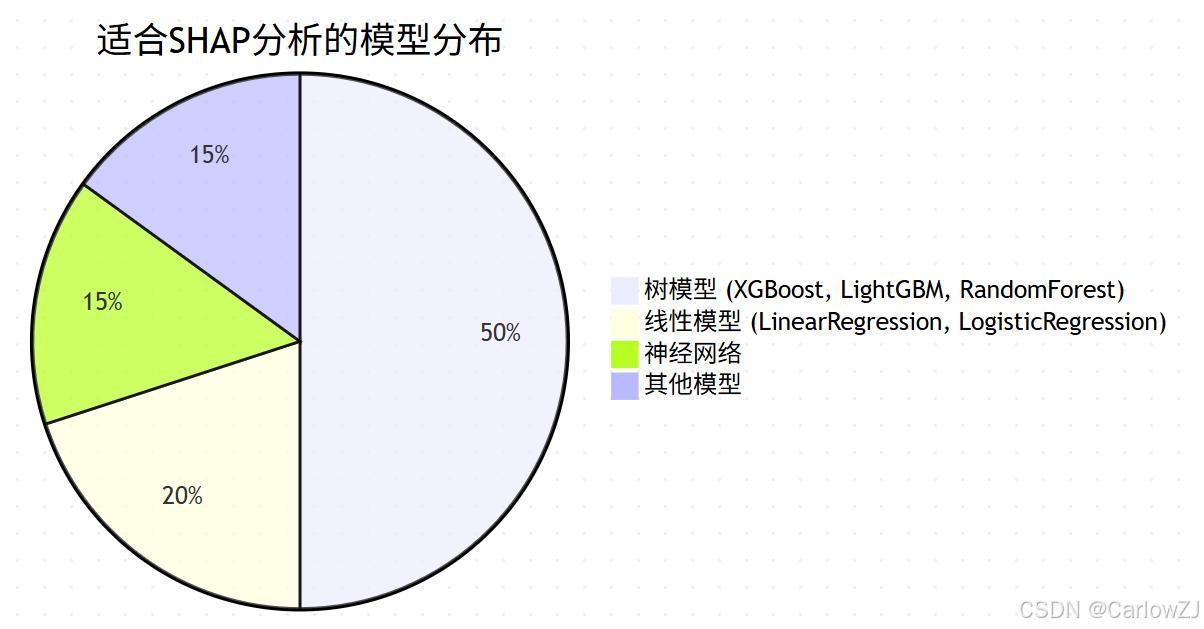
TreeExplainer：针对树模型（如XGBoost、LightGBM、Random Forest）的快速精确算法
LinearExplainer：针对线性模型的特化方法
DeepExplainer：针对深度神经网络的近似方法
KernelExplainer：适用于任何模型的模型无关方法

2. 多输出回归任务中的SHAP应用

在多输出回归任务中，模型需要同时预测多个连续目标变量。例如，预测房屋的多个属性（价格、租金、物业费）或预测客户的多个指标（收入、支出、储蓄）。

2.1 多输出回归SHAP分析原理

对于多输出回归任务，SHAP会为每个输出变量单独计算SHAP值。这意味着如果有n个特征和m个输出变量，我们将得到一个形状为(m, n, samples)的SHAP值数组。

2.2 实践示例：房价预测

让我们通过一个完整的示例来演示如何在多输出回归任务中应用SHAP分析。

import numpy as np
import pandas as pd
import matplotlib.pyplot as plt
import seaborn as sns
import xgboost as xgb
import shap
from sklearn.model_selection import train_test_split
from sklearn.metrics import mean_squared_error, r2_score
import warnings
warnings.filterwarnings('ignore')

# 设置中文字体和图形样式
plt.rcParams['font.sans-serif'] = ['SimHei']
plt.rcParams['axes.unicode_minus'] = False
sns.set_style("whitegrid")

def generate_house_data(n_samples=1000):
    """
    生成房屋数据集，包含多个目标变量
    """
    np.random.seed(42)
    
    # 生成特征
    area = np.random.normal(100, 30, n_samples)  # 面积（平方米）
    rooms = np.random.randint(1, 6, n_samples)   # 房间数
    age = np.random.randint(0, 50, n_samples)    # 房龄（年）
    location_score = np.random.uniform(1, 10, n_samples)  # 位置评分
    
    # 生成目标变量（多输出）
    # 房价（万元）
    price = (area * 0.5 + 
             rooms * 10 + 
             (10 - age/5) + 
             location_score * 8 + 
             np.random.normal(0, 5, n_samples))
    
    # 租金（万元/年）
    rent = (area * 0.03 + 
            rooms * 1.5 + 
            (5 - age/10) + 
            location_score * 1.2 + 
            np.random.normal(0, 1, n_samples))
    
    # 物业费（元/月）
    property_fee = (area * 0.1 + 
                   rooms * 2 + 
                   np.random.normal(0, 10, n_samples))
    
    # 创建DataFrame
    data = pd.DataFrame({
        'area': area,
        'rooms': rooms,
        'age': age,
        'location_score': location_score,
        'price': price,
        'rent': rent,
        'property_fee': property_fee
    })
    
    return data

# 生成数据
print("正在生成房屋数据集...")
house_data = generate_house_data(1000)
print(f"数据集形状: {house_data.shape}")
print("\n数据集前5行:")
print(house_data.head())

# 准备特征和目标变量
X = house_data[['area', 'rooms', 'age', 'location_score']]
y = house_data[['price', 'rent', 'property_fee']]

print(f"\n特征变量: {list(X.columns)}")
print(f"目标变量: {list(y.columns)}")

# 划分训练集和测试集
X_train, X_test, y_train, y_test = train_test_split(
    X, y, test_size=0.2, random_state=42
)

print(f"\n训练集大小: {X_train.shape}")
print(f"测试集大小: {X_test.shape}")

# 训练多输出回归模型
print("\n正在训练XGBoost多输出回归模型...")
model = xgb.XGBRegressor(
    n_estimators=100,
    max_depth=6,
    learning_rate=0.1,
    random_state=42
)

# 训练模型
model.fit(X_train, y_train)

# 预测
y_pred = model.predict(X_test)

# 评估模型性能
print("\n模型性能评估:")
for i, target in enumerate(y.columns):
    mse = mean_squared_error(y_test.iloc[:, i], y_pred[:, i])
    r2 = r2_score(y_test.iloc[:, i], y_pred[:, i])
    print(f"{target}: MSE = {mse:.2f}, R² = {r2:.4f}")

# SHAP分析
print("\n正在进行SHAP分析...")
explainer = shap.TreeExplainer(model)
shap_values = explainer.shap_values(X_train)

print(f"SHAP值形状: {np.array(shap_values).shape}")
print(f"目标变量数量: {len(shap_values)}")

2.3 多输出回归SHAP可视化

# 为每个目标变量创建SHAP分析
target_names = y.columns.tolist()

# 创建图形
fig, axes = plt.subplots(1, 3, figsize=(18, 5))

for i, (target_name, shap_value) in enumerate(zip(target_names, shap_values)):
    # 创建SHAP摘要图
    shap.summary_plot(
        shap_value, 
        X_train, 
        feature_names=X_train.columns,
        show=False,
        plot_size=None
    )
    plt.suptitle(f'{target_name} SHAP分析', fontsize=16)
    plt.tight_layout()
    plt.savefig(f'{target_name}_shap_summary.png', dpi=300, bbox_inches='tight')
    plt.show()

# 全局特征重要性分析
print("\n各目标变量的全局特征重要性:")
for i, target_name in enumerate(target_names):
    # 计算平均绝对SHAP值作为特征重要性
    feature_importance = np.mean(np.abs(shap_values[i]), axis=0)
    
    # 创建重要性DataFrame
    importance_df = pd.DataFrame({
        'feature': X_train.columns,
        'importance': feature_importance
    }).sort_values('importance', ascending=False)
    
    print(f"\n{target_name}:")
    print(importance_df)

2.4 局部解释分析

# 选择单个样本进行详细分析
sample_idx = 0
sample_data = X_train.iloc[sample_idx:sample_idx+1]

print("样本特征值:")
print(sample_data)

# 为每个目标变量生成力图
for i, target_name in enumerate(target_names):
    # 创建力图解释单个预测
    shap.initjs()
    shap.force_plot(
        explainer.expected_value[i],
        shap_values[i][sample_idx,:],
        X_train.iloc[sample_idx,:],
        feature_names=X_train.columns,
        matplotlib=True,
        show=False
    )
    plt.title(f'{target_name} 预测解释 (样本 #{sample_idx})')
    plt.tight_layout()
    plt.savefig(f'{target_name}_force_plot_sample_{sample_idx}.png', dpi=300, bbox_inches='tight')
    plt.show()

2.5 注意事项

在多输出回归任务中使用SHAP时需要注意以下几点：

独立计算：每个目标变量的SHAP值是独立计算的
结果解释：需要分别解释每个目标变量的特征贡献
计算复杂度：随着目标变量数量增加，计算量也会增加

3. 多分类任务中的SHAP应用

多分类任务是机器学习中的常见场景，如客户分类、图像识别、文本分类等。SHAP在多分类任务中的应用可以帮助我们理解模型对不同类别的决策过程。

3.1 多分类SHAP分析原理

在多分类任务中，SHAP会为每个类别生成一组SHAP值。对于n个特征和m个类别，我们将得到一个形状为(m, samples, n)的SHAP值数组。

3.2 实践示例：客户分类

让我们通过一个客户分类的示例来演示SHAP在多分类任务中的应用。

import numpy as np
import pandas as pd
import matplotlib.pyplot as plt
import seaborn as sns
import xgboost as xgb
import shap
from sklearn.model_selection import train_test_split
from sklearn.metrics import classification_report, confusion_matrix
from sklearn.preprocessing import LabelEncoder
import warnings
warnings.filterwarnings('ignore')

# 设置中文字体和图形样式
plt.rcParams['font.sans-serif'] = ['SimHei']
plt.rcParams['axes.unicode_minus'] = False
sns.set_style("whitegrid")

def generate_customer_data(n_samples=1000):
    """
    生成客户分类数据集
    """
    np.random.seed(42)
    
    # 生成特征
    age = np.random.randint(18, 80, n_samples)           # 年龄
    income = np.random.normal(50000, 20000, n_samples)   # 收入
    spending_score = np.random.uniform(1, 100, n_samples)  # 消费评分
    loyalty_years = np.random.randint(0, 20, n_samples)  # 忠诚度（年）
    
    # 生成客户类别（基于特征）
    customer_type = []
    for i in range(n_samples):
        # 基于规则生成客户类型
        score = (spending_score[i] * 0.4 + 
                income[i]/1000 * 0.3 + 
                loyalty_years[i] * 2 + 
                (80 - age[i]) * 0.1)
        
        if score > 60:
            customer_type.append('高价值客户')
        elif score > 30:
            customer_type.append('中价值客户')
        else:
            customer_type.append('低价值客户')
    
    # 创建DataFrame
    data = pd.DataFrame({
        'age': age,
        'income': income,
        'spending_score': spending_score,
        'loyalty_years': loyalty_years,
        'customer_type': customer_type
    })
    
    return data

# 生成数据
print("正在生成客户数据集...")
customer_data = generate_customer_data(1000)
print(f"数据集形状: {customer_data.shape}")
print("\n数据集前5行:")
print(customer_data.head())

# 查看类别分布
print("\n客户类型分布:")
print(customer_data['customer_type'].value_counts())

# 准备特征和目标变量
X = customer_data[['age', 'income', 'spending_score', 'loyalty_years']]
y = customer_data['customer_type']

# 编码目标变量
label_encoder = LabelEncoder()
y_encoded = label_encoder.fit_transform(y)
class_names = label_encoder.classes_

print(f"\n类别编码映射: {dict(zip(range(len(class_names)), class_names))}")

# 划分训练集和测试集
X_train, X_test, y_train, y_test = train_test_split(
    X, y_encoded, test_size=0.2, random_state=42, stratify=y_encoded
)

print(f"\n训练集大小: {X_train.shape}")
print(f"测试集大小: {X_test.shape}")

# 训练多分类模型
print("\n正在训练XGBoost多分类模型...")
model = xgb.XGBClassifier(
    objective='multi:softprob',  # 多分类概率输出
    num_class=len(class_names),  # 类别数量
    n_estimators=100,
    max_depth=6,
    learning_rate=0.1,
    random_state=42
)

# 训练模型
model.fit(X_train, y_train)

# 预测
y_pred = model.predict(X_test)
y_pred_proba = model.predict_proba(X_test)

# 评估模型性能
print("\n模型性能评估:")
print(classification_report(y_test, y_pred, target_names=class_names))

# 混淆矩阵
cm = confusion_matrix(y_test, y_pred)
plt.figure(figsize=(8, 6))
sns.heatmap(cm, annot=True, fmt='d', cmap='Blues', 
            xticklabels=class_names, yticklabels=class_names)
plt.title('混淆矩阵')
plt.xlabel('预测类别')
plt.ylabel('真实类别')
plt.tight_layout()
plt.savefig('confusion_matrix.png', dpi=300, bbox_inches='tight')
plt.show()

# SHAP分析
print("\n正在进行SHAP分析...")
explainer = shap.TreeExplainer(model)
shap_values = explainer.shap_values(X_train)

print(f"SHAP值形状: {np.array(shap_values).shape}")
print(f"类别数量: {len(shap_values)}")

3.3 多分类SHAP可视化

# 为每个类别创建SHAP分析
# 创建图形
fig, axes = plt.subplots(1, len(class_names), figsize=(20, 5))

for i, (class_name, shap_value) in enumerate(zip(class_names, shap_values)):
    # 创建SHAP摘要图
    shap.summary_plot(
        shap_value, 
        X_train, 
        feature_names=X_train.columns,
        show=False,
        plot_size=None
    )
    plt.title(f'{class_name} SHAP分析')
    plt.tight_layout()
    plt.savefig(f'{class_name}_shap_summary.png', dpi=300, bbox_inches='tight')
    plt.show()

# 全局特征重要性分析
print("\n各类别的全局特征重要性:")
for i, class_name in enumerate(class_names):
    # 计算平均绝对SHAP值作为特征重要性
    feature_importance = np.mean(np.abs(shap_values[i]), axis=0)
    
    # 创建重要性DataFrame
    importance_df = pd.DataFrame({
        'feature': X_train.columns,
        'importance': feature_importance
    }).sort_values('importance', ascending=False)
    
    print(f"\n{class_name}:")
    print(importance_df)

3.4 局部解释分析

# 选择单个样本进行详细分析
sample_idx = 0
sample_data = X_train.iloc[sample_idx:sample_idx+1]
sample_true_class = label_encoder.inverse_transform([y_train[sample_idx]])[0]

print(f"样本真实类别: {sample_true_class}")
print("样本特征值:")
print(sample_data)

# 获取预测概率
sample_pred_proba = model.predict_proba(sample_data)[0]
sample_pred_class_idx = np.argmax(sample_pred_proba)
sample_pred_class = label_encoder.inverse_transform([sample_pred_class_idx])[0]

print(f"预测类别: {sample_pred_class}")
print("各类别预测概率:")
for i, class_name in enumerate(class_names):
    print(f"  {class_name}: {sample_pred_proba[i]:.4f}")

# 为每个类别生成力图
for i, class_name in enumerate(class_names):
    # 创建力图解释单个预测
    shap.initjs()
    shap.force_plot(
        explainer.expected_value[i],
        shap_values[i][sample_idx,:],
        X_train.iloc[sample_idx,:],
        feature_names=X_train.columns,
        matplotlib=True,
        show=False
    )
    plt.title(f'{class_name} 预测解释 (样本 #{sample_idx})')
    plt.tight_layout()
    plt.savefig(f'{class_name}_force_plot_sample_{sample_idx}.png', dpi=300, bbox_inches='tight')
    plt.show()

3.5 类别间特征重要性对比

# 比较不同类别间的特征重要性
feature_importance_comparison = pd.DataFrame()

for i, class_name in enumerate(class_names):
    importance = np.mean(np.abs(shap_values[i]), axis=0)
    feature_importance_comparison[class_name] = importance

feature_importance_comparison.index = X_train.columns
print("\n各类别特征重要性对比:")
print(feature_importance_comparison)

# 可视化特征重要性对比
plt.figure(figsize=(12, 8))
feature_importance_comparison.plot(kind='bar', figsize=(12, 8))
plt.title('各类别特征重要性对比')
plt.xlabel('特征')
plt.ylabel('平均|SHAP值|')
plt.legend(title='客户类别')
plt.xticks(rotation=45)
plt.tight_layout()
plt.savefig('feature_importance_comparison.png', dpi=300, bbox_inches='tight')
plt.show()

3.6 注意事项

在多分类任务中使用SHAP时需要注意以下几点：

一次性输出：SHAP值会为每个类别生成一个矩阵
概率输出：确保模型输出概率而非类别标签
类别平衡：注意类别不平衡对SHAP分析的影响

4. SHAP高级可视化技术

SHAP提供了丰富的可视化工具，帮助我们更好地理解模型的决策过程。

4.1 Summary Plot（摘要图）

# 创建综合摘要图
def create_comprehensive_summary(shap_values, X_train, class_names=None, target_names=None):
    """
    创建综合SHAP摘要图
    """
    if class_names is not None:
        # 多分类情况
        for i, class_name in enumerate(class_names):
            plt.figure(figsize=(10, 6))
            shap.summary_plot(
                shap_values[i], 
                X_train, 
                feature_names=X_train.columns,
                show=False
            )
            plt.title(f'{class_name} - SHAP特征重要性摘要')
            plt.tight_layout()
            plt.savefig(f'{class_name}_summary_plot.png', dpi=300, bbox_inches='tight')
            plt.show()
    elif target_names is not None:
        # 多输出回归情况
        for i, target_name in enumerate(target_names):
            plt.figure(figsize=(10, 6))
            shap.summary_plot(
                shap_values[i], 
                X_train, 
                feature_names=X_train.columns,
                show=False
            )
            plt.title(f'{target_name} - SHAP特征重要性摘要')
            plt.tight_layout()
            plt.savefig(f'{target_name}_summary_plot.png', dpi=300, bbox_inches='tight')
            plt.show()

# 为多分类示例创建摘要图
create_comprehensive_summary(shap_values, X_train, class_names=class_names)

4.2 Dependence Plot（依赖图）

# 创建特征依赖图
def create_dependence_plots(shap_values, X_train, class_names=None, target_names=None):
    """
    为重要特征创建依赖图
    """
    if class_names is not None:
        # 多分类情况
        for i, class_name in enumerate(class_names):
            # 计算特征重要性
            feature_importance = np.mean(np.abs(shap_values[i]), axis=0)
            top_features_idx = np.argsort(feature_importance)[-3:]  # 取前3个重要特征
            
            for idx in top_features_idx:
                feature_name = X_train.columns[idx]
                plt.figure(figsize=(10, 6))
                shap.dependence_plot(
                    idx, 
                    shap_values[i], 
                    X_train,
                    show=False
                )
                plt.title(f'{class_name} - {feature_name} 依赖关系')
                plt.tight_layout()
                plt.savefig(f'{class_name}_{feature_name}_dependence.png', dpi=300, bbox_inches='tight')
                plt.show()
    elif target_names is not None:
        # 多输出回归情况
        for i, target_name in enumerate(target_names):
            # 计算特征重要性
            feature_importance = np.mean(np.abs(shap_values[i]), axis=0)
            top_features_idx = np.argsort(feature_importance)[-3:]  # 取前3个重要特征
            
            for idx in top_features_idx:
                feature_name = X_train.columns[idx]
                plt.figure(figsize=(10, 6))
                shap.dependence_plot(
                    idx, 
                    shap_values[i], 
                    X_train,
                    show=False
                )
                plt.title(f'{target_name} - {feature_name} 依赖关系')
                plt.tight_layout()
                plt.savefig(f'{target_name}_{feature_name}_dependence.png', dpi=300, bbox_inches='tight')
                plt.show()

# 为多分类示例创建依赖图
create_dependence_plots(shap_values, X_train, class_names=class_names)

4.3 Decision Plot（决策图）

# 创建决策图
def create_decision_plots(model, explainer, shap_values, X_train, X_test, 
                         y_test, label_encoder=None, class_names=None):
    """
    创建决策图展示模型决策过程
    """
    # 选择几个测试样本
    sample_indices = [0, 1, 2]
    
    for idx in sample_indices:
        sample_data = X_test.iloc[idx:idx+1]
        sample_true = y_test[idx]
        
        if label_encoder is not None:
            sample_true_label = label_encoder.inverse_transform([sample_true])[0]
        else:
            sample_true_label = sample_true
            
        print(f"\n样本 #{idx} 真实类别: {sample_true_label}")
        
        # 获取预测
        if hasattr(model, 'predict_proba'):
            pred_proba = model.predict_proba(sample_data)[0]
            predicted_class_idx = np.argmax(pred_proba)
            if label_encoder is not None:
                predicted_label = label_encoder.inverse_transform([predicted_class_idx])[0]
            else:
                predicted_label = predicted_class_idx
            print(f"预测类别: {predicted_label}")
            
        # 为预测类别创建决策图
        if class_names is not None:
            plt.figure(figsize=(12, 8))
            shap.decision_plot(
                explainer.expected_value[predicted_class_idx],
                shap_values[predicted_class_idx][idx:idx+1],
                X_test.iloc[idx:idx+1],
                feature_names=X_test.columns,
                show=False
            )
            plt.title(f'样本 #{idx} 决策过程 - 预测类别: {predicted_label}')
            plt.tight_layout()
            plt.savefig(f'decision_plot_sample_{idx}.png', dpi=300, bbox_inches='tight')
            plt.show()

# 为多分类示例创建决策图
create_decision_plots(model, explainer, shap_values, X_train, X_test, 
                     y_test, label_encoder, class_names)

5. 注意事项与最佳实践

5.1 注意事项

5.1.1 计算性能考虑

import time

def benchmark_shap_methods(X_train, model):
    """
    比较不同SHAP方法的性能
    """
    methods = {
        'TreeExplainer': lambda: shap.TreeExplainer(model),
        # 'KernelExplainer': lambda: shap.KernelExplainer(model.predict, X_train.iloc[:100])
    }
    
    results = {}
    
    for name, explainer_func in methods.items():
        try:
            start_time = time.time()
            explainer = explainer_func()
            explainer_time = time.time() - start_time
            
            start_time = time.time()
            shap_values = explainer.shap_values(X_train.iloc[:100])
            calculation_time = time.time() - start_time
            
            results[name] = {
                'explainer_time': explainer_time,
                'calculation_time': calculation_time,
                'total_time': explainer_time + calculation_time
            }
            
            print(f"{name}:")
            print(f"  Explainer创建时间: {explainer_time:.4f}秒")
            print(f"  SHAP值计算时间: {calculation_time:.4f}秒")
            print(f"  总时间: {explainer_time + calculation_time:.4f}秒")
            
        except Exception as e:
            print(f"{name} 失败: {e}")
    
    return results

# 性能基准测试
print("正在进行SHAP方法性能基准测试...")
benchmark_results = benchmark_shap_methods(X_train, model)

5.1.2 数据质量影响

def analyze_data_quality_impact(X_train):
    """
    分析数据质量对SHAP分析的影响
    """
    print("数据质量分析:")
    print(f"数据集形状: {X_train.shape}")
    print(f"缺失值统计:")
    print(X_train.isnull().sum())
    
    print(f"\n数据类型:")
    print(X_train.dtypes)
    
    print(f"\n数值特征统计:")
    print(X_train.describe())

# 分析数据质量
analyze_data_quality_impact(X_train)

5.2 最佳实践

5.2.1 模型选择建议

在这里插入图片描述

5.2.2 特征工程优化

def feature_engineering_best_practices(X):
    """
    特征工程最佳实践
    """
    print("特征工程建议:")
    print("1. 处理缺失值:")
    missing_ratio = X.isnull().sum() / len(X)
    high_missing_features = missing_ratio[missing_ratio > 0.5].index.tolist()
    if high_missing_features:
        print(f"   高缺失率特征 (>50%): {high_missing_features}")
    
    print("\n2. 处理异常值:")
    numeric_features = X.select_dtypes(include=[np.number]).columns
    for feature in numeric_features:
        Q1 = X[feature].quantile(0.25)
        Q3 = X[feature].quantile(0.75)
        IQR = Q3 - Q1
        lower_bound = Q1 - 1.5 * IQR
        upper_bound = Q3 + 1.5 * IQR
        outliers = X[(X[feature] < lower_bound) | (X[feature] > upper_bound)]
        outlier_ratio = len(outliers) / len(X)
        if outlier_ratio > 0.05:  # 超过5%的异常值
            print(f"   {feature}: 异常值比例 {outlier_ratio:.2%}")
    
    print("\n3. 特征缩放:")
    print("   对于线性模型，建议进行特征标准化")
    print("   对于树模型，通常不需要特征缩放")

# 应用特征工程最佳实践
feature_engineering_best_practices(X_train)

5.2.3 结果验证方法

def validate_shap_results(model, explainer, shap_values, X_test, y_test, 
                         label_encoder=None, class_names=None):
    """
    验证SHAP分析结果的合理性
    """
    print("SHAP结果验证:")
    
    # 1. 检查SHAP值的一致性
    if class_names is not None:
        # 多分类情况
        for i, class_name in enumerate(class_names):
            shap_sum = np.sum(shap_values[i], axis=1)
            expected_range = explainer.expected_value[i]
            print(f"{class_name} - SHAP值一致性检查:")
            print(f"  平均SHAP值总和: {np.mean(shap_sum):.4f}")
            print(f"  基准值: {expected_range:.4f}")
            print(f"  差异: {abs(np.mean(shap_sum) - expected_range):.4f}")
    
    # 2. 检查特征重要性稳定性
    print("\n特征重要性稳定性检查:")
    if class_names is not None:
        # 计算不同样本子集的特征重要性
        subset1_indices = np.random.choice(len(X_test), len(X_test)//2, replace=False)
        subset2_indices = np.setdiff1d(np.arange(len(X_test)), subset1_indices)
        
        for i, class_name in enumerate(class_names):
            importance1 = np.mean(np.abs(shap_values[i][subset1_indices]), axis=0)
            importance2 = np.mean(np.abs(shap_values[i][subset2_indices]), axis=0)
            
            # 计算相关性
            correlation = np.corrcoef(importance1, importance2)[0, 1]
            print(f"  {class_name} 特征重要性稳定性 (相关系数): {correlation:.4f}")

# 验证SHAP结果
validate_shap_results(model, explainer, shap_values, X_test, y_test, 
                     label_encoder, class_names)

6. 常见问题解答

6.1 SHAP是否支持多目标变量？

是的，SHAP支持多输出回归和多分类任务：

多输出回归：为每个目标变量单独计算SHAP值
多分类：为每个类别生成一组SHAP值
多标签分类：可以视为多输出回归任务处理

6.2 如何处理多输出回归任务？

对于多输出回归任务，需要：

使用支持多输出的模型（如XGBoost的多输出回归）
为每个目标变量单独计算SHAP值
分别解释每个目标变量的特征贡献

# 多输出回归SHAP处理示例
def multi_output_shap_example():
    """
    多输出回归SHAP处理示例
    """
    print("多输出回归SHAP处理步骤:")
    print("1. 训练多输出回归模型")
    print("2. 创建SHAP解释器")
    print("3. 计算SHAP值（会为每个输出变量返回一个SHAP值数组）")
    print("4. 分别分析每个输出变量的特征重要性")
    print("5. 可视化每个输出变量的SHAP摘要图")

multi_output_shap_example()

6.3 如何处理多分类任务？

对于多分类任务，需要：

确保模型输出概率而非类别标签
SHAP会为每个类别生成一组SHAP值
可以选择特定类别进行详细分析

# 多分类SHAP处理示例
def multi_class_shap_example():
    """
    多分类SHAP处理示例
    """
    print("多分类SHAP处理步骤:")
    print("1. 训练多分类模型（确保输出概率）")
    print("2. 创建SHAP解释器")
    print("3. 计算SHAP值（会为每个类别返回一个SHAP值数组）")
    print("4. 分析每个类别的特征重要性")
    print("5. 可视化各类别的SHAP摘要图")

multi_class_shap_example()

6.4 SHAP计算很慢怎么办？

SHAP计算慢的解决方案：

def optimize_shap_performance():
    """
    SHAP性能优化建议
    """
    print("SHAP性能优化建议:")
    print("1. 选择合适的解释器:")
    print("   - TreeExplainer: 适用于树模型（最快）")
    print("   - LinearExplainer: 适用于线性模型")
    print("   - DeepExplainer: 适用于深度学习模型")
    print("   - KernelExplainer: 通用但较慢")
    
    print("\n2. 减少样本数量:")
    print("   - 对于大数据集，可以采样部分数据进行SHAP分析")
    
    print("\n3. 减少特征数量:")
    print("   - 只分析重要特征的SHAP值")
    
    print("\n4. 并行计算:")
    print("   - 某些SHAP解释器支持并行计算")

optimize_shap_performance()

6.5 SHAP值如何解释？

SHAP值的解释：

正值：特征值推动预测向更高值发展
负值：特征值推动预测向更低值发展
零值：特征值对预测没有影响
绝对值大小：表示特征影响的强度

def interpret_shap_values_example():
    """
    SHAP值解释示例
    """
    print("SHAP值解释示例:")
    print("假设SHAP值为:")
    print("  年龄: -0.5 (年龄越大，预测值越低)")
    print("  收入: +1.2 (收入越高，预测值越高)")
    print("  消费评分: +0.8 (消费评分越高，预测值越高)")
    print("  忠诚度: +0.3 (忠诚度越高，预测值越高)")
    print("\n结论: 收入是对预测影响最大的特征")

interpret_shap_values_example()

7. 扩展阅读

7.1 相关工具和库

7.2 高级应用案例

医疗诊断：解释疾病预测模型的决策依据
金融风控：分析信贷审批模型的风险因素
推荐系统：理解用户偏好预测的驱动因素
图像识别：解释CNN模型的视觉注意力机制

7.3 研究前沿

SHAP值的不确定性量化
因果推理与SHAP的结合
大规模数据的SHAP近似算法
SHAP在强化学习中的应用

实施计划甘特图

交互流程时序图

总结

本文全面介绍了SHAP分析在多目标变量场景下的应用，包括多输出回归和多分类任务。通过深入的理论讲解和丰富的实践示例，我们掌握了以下关键要点：

关键要点回顾

理论基础：SHAP基于博弈论中的Shapley值，为每个特征分配贡献值，具有公平性、局部解释性和全局解释性等特点。
多输出回归应用：为每个目标变量独立计算SHAP值，能够分别解释各目标变量的特征贡献。
多分类应用：为每个类别生成一组SHAP值，帮助理解模型对不同类别的决策过程。
可视化技术：通过摘要图、依赖图、决策图等多种可视化手段，直观展示模型的决策机制。
最佳实践：包括模型选择、特征工程、结果验证等方面的建议，确保SHAP分析的有效性和可靠性。

实践建议

选择合适的解释器：根据模型类型选择最适合的SHAP解释器，如TreeExplainer用于树模型。
关注计算性能：对于大数据集或复杂模型，需要考虑计算效率和资源消耗。
验证结果合理性：通过多种方法验证SHAP分析结果的准确性和一致性。
结合业务理解：将SHAP分析结果与业务知识结合，提供有价值的洞察。

未来展望

随着机器学习模型在各行各业的广泛应用，模型可解释性将变得越来越重要。SHAP作为一种强大的解释工具，将在以下方面继续发展：

算法优化：提高SHAP值计算的效率和准确性
应用扩展：拓展到更多类型的模型和任务
工具集成：与其他机器学习工具和平台更好地集成
标准制定：建立行业标准和最佳实践指南

通过正确应用SHAP分析，我们可以更好地理解和信任机器学习模型，为业务决策提供有力支持，同时满足监管和合规要求。

参考资料

Lundberg, S. M., & Lee, S. I. (2017). A unified approach to interpreting model predictions. Advances in neural information processing systems, 30.
SHAP官方文档
XGBoost官方文档
LightGBM官方文档
Molnar, C. (2020). Interpretable machine learning. Lulu.com.
SHAP GitHub仓库
可解释AI综述
Guidotti, R., Monreale, A., Ruggieri, S., Turini, F., Giannotti, F., & Pedreschi, D. (2018). A survey of methods for explaining black box models. ACM computing surveys (CSUR), 51(5), 1-42.
机器学习可解释性工具比较
博弈论与机器学习