


1. Softmax回归
① Softmax回归虽然它的名字是回归,其实它是一个分类问题。

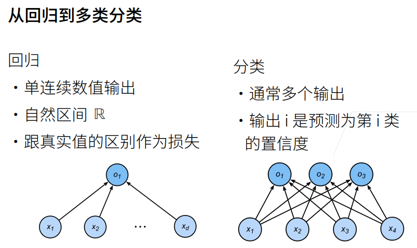
2. 回归VS分类

3. Kaggle分类问题


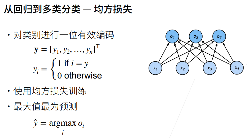
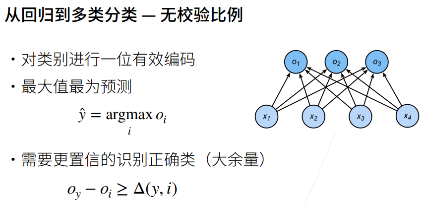
4. 回归到分类
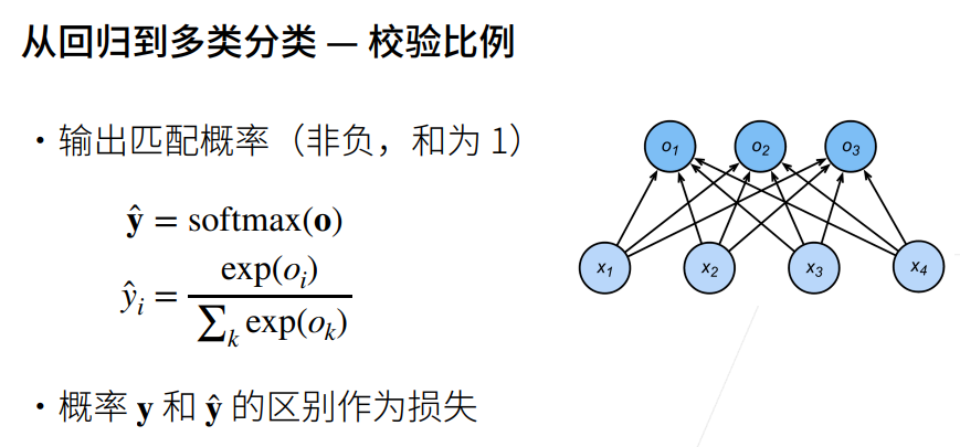
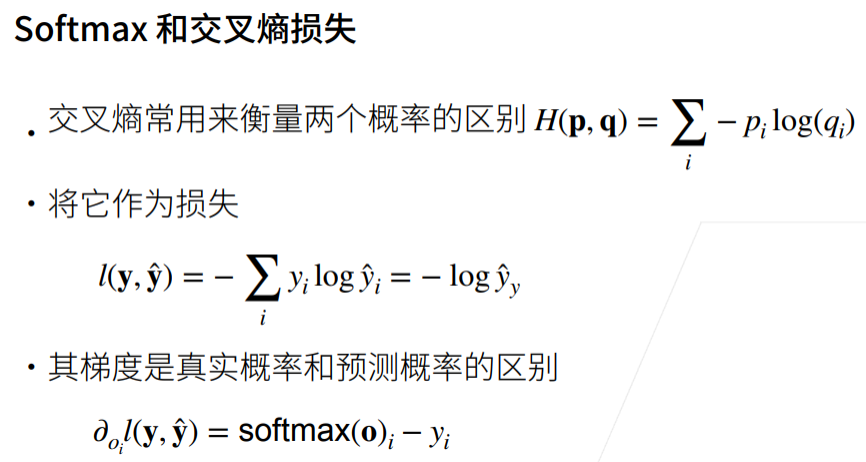
5. 交叉熵损失
6. 总结

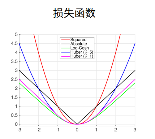
7. 损失函数
① 三个常用的损失函数 L2 loss、L1 loss、Huber’s Robust loss。
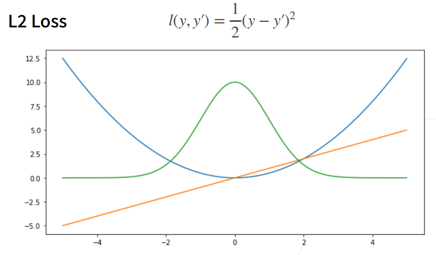
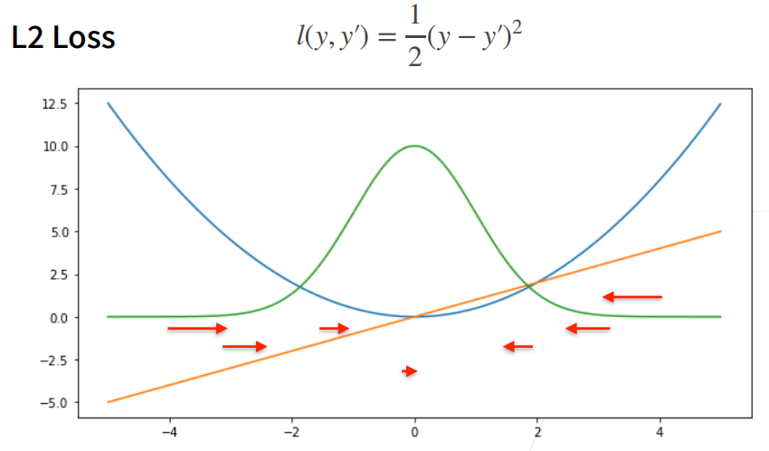
8. L2 Loss
① 蓝色曲线为当y=0时,变换y’所获得的曲线。
② 绿色曲线为当y=0时,变换y’所获得的曲线的似然函数,即1−l(y,y′)1^{-l(y,y')}1−l(y,y′),似然函数呈高斯分布。最小化损失函数就是最大化似然函数。
③ 橙色曲线为损失函数的梯度,梯度是一次函数,所以穿过原点。
④ 当预测值y’跟真实值y隔的比较远的时候,(真实值y为0,预测值就是下面的曲线里的x轴),梯度比较大,所以参数更新比较多。
⑤ 随着预测值靠近真实值是,梯度越来越小,参数的更新越来越小。
9. L1 Loss
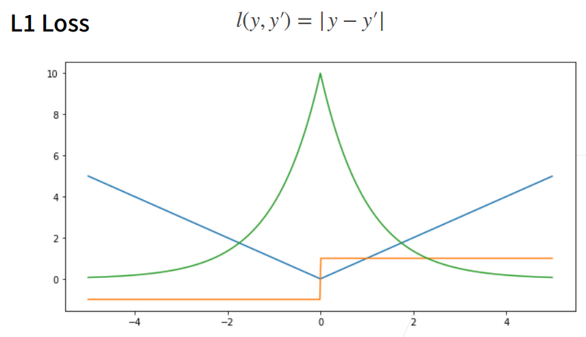
① 相对L2 loss,L1 loss的梯度就是距离原点时,梯度也不是特别大,权重的更新也不是特别大。会带来很多稳定性的好处。
② 他的缺点是在零点处不可导,并在零点处左右有±1的变化,这个不平滑性导致预测值与真实值靠的比较近的时候,优化到末期的时候,可能会不那么稳定。

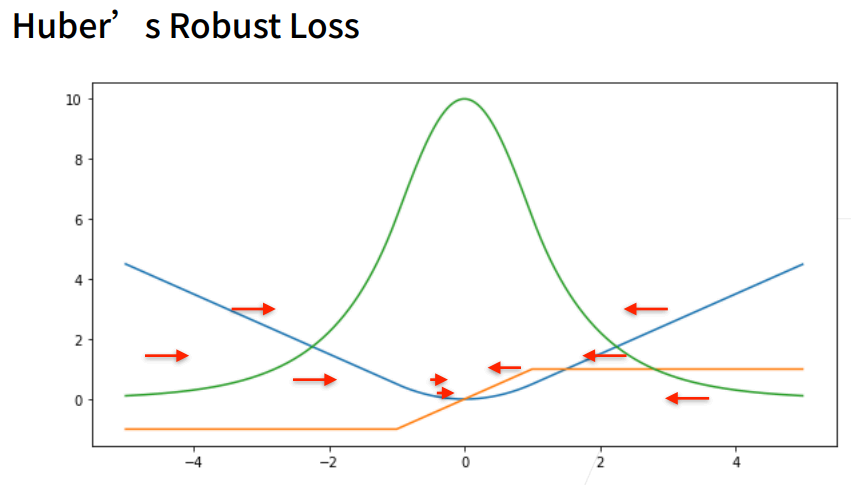
10. Huber’s Robust Loss
① 结合L1 loss 和L2 loss损失。

1. 图像分类数据集
① MINIST数据集是图像分类中广泛使用的数据集之一,但作为基准数据集过于简单。
② 下面将使用类似但更复杂的Fashion-MNIST数据集。
1.1 显示图片
%matplotlib inline
import torch
import torchvision
from torch.utils import data
from torchvision import transforms
from d2l import torch as d2l

# SVG是一种无损格式 – 意味着它在压缩时不会丢失任何数据,可以呈现无限数量的颜色。
# SVG最常用于网络上的图形、徽标可供其他高分辨率屏幕上查看。
d2l.use_svg_display() # 使用svg来显示图片,这样清晰度高一些。
help(d2l.use_svg_display)
Help on function use_svg_display in module d2l.torch:

use_svg_display()
    Use the svg format to display a plot in Jupyter.
1.2 数据集下载
%matplotlib inline
import torch
import torchvision
from torch.utils import data
from torchvision import transforms
from d2l import torch as d2l

d2l.use_svg_display()

# 通过ToTensor实例将图像数据从PIL类型变换成32位浮点数格式
# 并除以255使得所有像素的数值均在0到1之间
trans = transforms.ToTensor()
mnist_train = torchvision.datasets.FashionMNIST(root="01_data/01_DataSet_FashionMNIST",train=True,transform=trans,download=True)
mnist_test = torchvision.datasets.FashionMNIST(root="01_data/01_DataSet_FashionMNIST",train=False,transform=trans,download=True)
print(len(mnist_train)) # 训练数据集长度
print(len(mnist_test))  # 测试数据集长度

print(mnist_train[0][0].shape) # 黑白图片,所以channel为1。
print(mnist_train[0][1]) # [0][0]表示第一个样本的图片信息,[0][1]表示该样本对应的标签值
60000
10000
torch.Size([1, 28, 28])
9
1.3 可视化数据集
%matplotlib inline
import torch
import torchvision
from torch.utils import data
from torchvision import transforms
from d2l import torch as d2l

d2l.use_svg_display()

# 通过ToTensor实例将图像数据从PIL类型变换成32位浮点数格式
# 并除以255使得所有像素的数值均在0到1之间
trans = transforms.ToTensor()
mnist_train = torchvision.datasets.FashionMNIST(root="01_data/01_DataSet_FashionMNIST",train=True,transform=trans,download=True)
mnist_test = torchvision.datasets.FashionMNIST(root="01_data/01_DataSet_FashionMNIST",train=False,transform=trans,download=True)

def get_fashion_mnist_labels(labels):
    """返回Fashion-MNIST数据集的文本标签"""
    text_labels = ['t-shirt','trouser','pullover','dress','coat',
                   'sandal','shirt','sneaker','bag','ankle boot']
    return [text_labels[int(i)] for i in labels]

def show_images(imgs, num_rows, num_cols, titles=None, scale=1.5):
    """Plot a list of images."""
    figsize = (num_cols * scale, num_rows * scale) # 传进来的图像尺寸,scale 为放缩比例因子
    _, axes = d2l.plt.subplots(num_rows,num_cols,figsize=figsize)
    print(_)
    print(axes) # axes 为构建的两行九列的画布
    axes = axes.flatten()
    print(axes) # axes 变成一维数据
    for i,(ax,img) in enumerate(zip(axes,imgs)):
        if(i<1):
            print("i:",i)
            print("ax,img:",ax,img)
        if torch.is_tensor(img):
            # 图片张量
            ax.imshow(img.numpy())
            ax.set_title(titles[i])
        else:
            # PIL图片
            ax.imshow(img)

X, y = next(iter(data.DataLoader(mnist_train,batch_size=18))) # X,y 为仅抽取一次的18个样本的图片、以及对应的标签值
show_images(X.reshape(18,28,28),2,9,titles=get_fashion_mnist_labels(y))
Figure(972x216)
[[<AxesSubplot:> <AxesSubplot:> <AxesSubplot:> <AxesSubplot:>
  <AxesSubplot:> <AxesSubplot:> <AxesSubplot:> <AxesSubplot:>
  <AxesSubplot:>]
 [<AxesSubplot:> <AxesSubplot:> <AxesSubplot:> <AxesSubplot:>
  <AxesSubplot:> <AxesSubplot:> <AxesSubplot:> <AxesSubplot:>
  <AxesSubplot:>]]
[<AxesSubplot:> <AxesSubplot:> <AxesSubplot:> <AxesSubplot:>
 <AxesSubplot:> <AxesSubplot:> <AxesSubplot:> <AxesSubplot:>
 <AxesSubplot:> <AxesSubplot:> <AxesSubplot:> <AxesSubplot:>
 <AxesSubplot:> <AxesSubplot:> <AxesSubplot:> <AxesSubplot:>
 <AxesSubplot:> <AxesSubplot:>]
i: 0
ax,img: AxesSubplot(0.125,0.536818;0.0731132x0.343182) tensor([[0.0000, 0.0000, 0.0000, 0.0000, 0.0000, 0.0000, 0.0000, 0.0000, 0.0000,
         0.0000, 0.0000, 0.0000, 0.0000, 0.0000, 0.0000, 0.0000, 0.0000, 0.0000,
         0.0000, 0.0000, 0.0000, 0.0000, 0.0000, 0.0000, 0.0000, 0.0000, 0.0000,
         0.0000],
        [0.0000, 0.0000, 0.0000, 0.0000, 0.0000, 0.0000, 0.0000, 0.0000, 0.0000,
         0.0000, 0.0000, 0.0000, 0.0000, 0.0000, 0.0000, 0.0000, 0.0000, 0.0000,
         0.0000, 0.0000, 0.0000, 0.0000, 0.0000, 0.0000, 0.0000, 0.0000, 0.0000,
         0.0000],
        [0.0000, 0.0000, 0.0000, 0.0000, 0.0000, 0.0000, 0.0000, 0.0000, 0.0000,
         0.0000, 0.0000, 0.0000, 0.0000, 0.0000, 0.0000, 0.0000, 0.0000, 0.0000,
         0.0000, 0.0000, 0.0000, 0.0000, 0.0000, 0.0000, 0.0000, 0.0000, 0.0000,
         0.0000],
        [0.0000, 0.0000, 0.0000, 0.0000, 0.0000, 0.0000, 0.0000, 0.0000, 0.0000,
         0.0000, 0.0000, 0.0000, 0.0039, 0.0000, 0.0000, 0.0510, 0.2863, 0.0000,
         0.0000, 0.0039, 0.0157, 0.0000, 0.0000, 0.0000, 0.0000, 0.0039, 0.0039,
         0.0000],
        [0.0000, 0.0000, 0.0000, 0.0000, 0.0000, 0.0000, 0.0000, 0.0000, 0.0000,
         0.0000, 0.0000, 0.0000, 0.0118, 0.0000, 0.1412, 0.5333, 0.4980, 0.2431,
         0.2118, 0.0000, 0.0000, 0.0000, 0.0039, 0.0118, 0.0157, 0.0000, 0.0000,
         0.0118],
        [0.0000, 0.0000, 0.0000, 0.0000, 0.0000, 0.0000, 0.0000, 0.0000, 0.0000,
         0.0000, 0.0000, 0.0000, 0.0235, 0.0000, 0.4000, 0.8000, 0.6902, 0.5255,
         0.5647, 0.4824, 0.0902, 0.0000, 0.0000, 0.0000, 0.0000, 0.0471, 0.0392,
         0.0000],
        [0.0000, 0.0000, 0.0000, 0.0000, 0.0000, 0.0000, 0.0000, 0.0000, 0.0000,
         0.0000, 0.0000, 0.0000, 0.0000, 0.0000, 0.6078, 0.9255, 0.8118, 0.6980,
         0.4196, 0.6118, 0.6314, 0.4275, 0.2510, 0.0902, 0.3020, 0.5098, 0.2824,
         0.0588],
        [0.0000, 0.0000, 0.0000, 0.0000, 0.0000, 0.0000, 0.0000, 0.0000, 0.0000,
         0.0000, 0.0000, 0.0039, 0.0000, 0.2706, 0.8118, 0.8745, 0.8549, 0.8471,
         0.8471, 0.6392, 0.4980, 0.4745, 0.4784, 0.5725, 0.5529, 0.3451, 0.6745,
         0.2588],
        [0.0000, 0.0000, 0.0000, 0.0000, 0.0000, 0.0000, 0.0000, 0.0000, 0.0000,
         0.0039, 0.0039, 0.0039, 0.0000, 0.7843, 0.9098, 0.9098, 0.9137, 0.8980,
         0.8745, 0.8745, 0.8431, 0.8353, 0.6431, 0.4980, 0.4824, 0.7686, 0.8980,
         0.0000],
        [0.0000, 0.0000, 0.0000, 0.0000, 0.0000, 0.0000, 0.0000, 0.0000, 0.0000,
         0.0000, 0.0000, 0.0000, 0.0000, 0.7176, 0.8824, 0.8471, 0.8745, 0.8941,
         0.9216, 0.8902, 0.8784, 0.8706, 0.8784, 0.8667, 0.8745, 0.9608, 0.6784,
         0.0000],
        [0.0000, 0.0000, 0.0000, 0.0000, 0.0000, 0.0000, 0.0000, 0.0000, 0.0000,
         0.0000, 0.0000, 0.0000, 0.0000, 0.7569, 0.8941, 0.8549, 0.8353, 0.7765,
         0.7059, 0.8314, 0.8235, 0.8275, 0.8353, 0.8745, 0.8627, 0.9529, 0.7922,
         0.0000],
        [0.0000, 0.0000, 0.0000, 0.0000, 0.0000, 0.0000, 0.0000, 0.0000, 0.0000,
         0.0039, 0.0118, 0.0000, 0.0471, 0.8588, 0.8627, 0.8314, 0.8549, 0.7529,
         0.6627, 0.8902, 0.8157, 0.8549, 0.8784, 0.8314, 0.8863, 0.7725, 0.8196,
         0.2039],
        [0.0000, 0.0000, 0.0000, 0.0000, 0.0000, 0.0000, 0.0000, 0.0000, 0.0000,
         0.0000, 0.0235, 0.0000, 0.3882, 0.9569, 0.8706, 0.8627, 0.8549, 0.7961,
         0.7765, 0.8667, 0.8431, 0.8353, 0.8706, 0.8627, 0.9608, 0.4667, 0.6549,
         0.2196],
        [0.0000, 0.0000, 0.0000, 0.0000, 0.0000, 0.0000, 0.0000, 0.0000, 0.0000,
         0.0157, 0.0000, 0.0000, 0.2157, 0.9255, 0.8941, 0.9020, 0.8941, 0.9412,
         0.9098, 0.8353, 0.8549, 0.8745, 0.9176, 0.8510, 0.8510, 0.8196, 0.3608,
         0.0000],
        [0.0000, 0.0000, 0.0039, 0.0157, 0.0235, 0.0275, 0.0078, 0.0000, 0.0000,
         0.0000, 0.0000, 0.0000, 0.9294, 0.8863, 0.8510, 0.8745, 0.8706, 0.8588,
         0.8706, 0.8667, 0.8471, 0.8745, 0.8980, 0.8431, 0.8549, 1.0000, 0.3020,
         0.0000],
        [0.0000, 0.0118, 0.0000, 0.0000, 0.0000, 0.0000, 0.0000, 0.0000, 0.0000,
         0.2431, 0.5686, 0.8000, 0.8941, 0.8118, 0.8353, 0.8667, 0.8549, 0.8157,
         0.8275, 0.8549, 0.8784, 0.8745, 0.8588, 0.8431, 0.8784, 0.9569, 0.6235,
         0.0000],
        [0.0000, 0.0000, 0.0000, 0.0000, 0.0706, 0.1725, 0.3216, 0.4196, 0.7412,
         0.8941, 0.8627, 0.8706, 0.8510, 0.8863, 0.7843, 0.8039, 0.8275, 0.9020,
         0.8784, 0.9176, 0.6902, 0.7373, 0.9804, 0.9725, 0.9137, 0.9333, 0.8431,
         0.0000],
        [0.0000, 0.2235, 0.7333, 0.8157, 0.8784, 0.8667, 0.8784, 0.8157, 0.8000,
         0.8392, 0.8157, 0.8196, 0.7843, 0.6235, 0.9608, 0.7569, 0.8078, 0.8745,
         1.0000, 1.0000, 0.8667, 0.9176, 0.8667, 0.8275, 0.8627, 0.9098, 0.9647,
         0.0000],
        [0.0118, 0.7922, 0.8941, 0.8784, 0.8667, 0.8275, 0.8275, 0.8392, 0.8039,
         0.8039, 0.8039, 0.8627, 0.9412, 0.3137, 0.5882, 1.0000, 0.8980, 0.8667,
         0.7373, 0.6039, 0.7490, 0.8235, 0.8000, 0.8196, 0.8706, 0.8941, 0.8824,
         0.0000],
        [0.3843, 0.9137, 0.7765, 0.8235, 0.8706, 0.8980, 0.8980, 0.9176, 0.9765,
         0.8627, 0.7608, 0.8431, 0.8510, 0.9451, 0.2549, 0.2863, 0.4157, 0.4588,
         0.6588, 0.8588, 0.8667, 0.8431, 0.8510, 0.8745, 0.8745, 0.8784, 0.8980,
         0.1137],
        [0.2941, 0.8000, 0.8314, 0.8000, 0.7569, 0.8039, 0.8275, 0.8824, 0.8471,
         0.7255, 0.7725, 0.8078, 0.7765, 0.8353, 0.9412, 0.7647, 0.8902, 0.9608,
         0.9373, 0.8745, 0.8549, 0.8314, 0.8196, 0.8706, 0.8627, 0.8667, 0.9020,
         0.2627],
        [0.1882, 0.7961, 0.7176, 0.7608, 0.8353, 0.7725, 0.7255, 0.7451, 0.7608,
         0.7529, 0.7922, 0.8392, 0.8588, 0.8667, 0.8627, 0.9255, 0.8824, 0.8471,
         0.7804, 0.8078, 0.7294, 0.7098, 0.6941, 0.6745, 0.7098, 0.8039, 0.8078,
         0.4510],
        [0.0000, 0.4784, 0.8588, 0.7569, 0.7020, 0.6706, 0.7176, 0.7686, 0.8000,
         0.8235, 0.8353, 0.8118, 0.8275, 0.8235, 0.7843, 0.7686, 0.7608, 0.7490,
         0.7647, 0.7490, 0.7765, 0.7529, 0.6902, 0.6118, 0.6549, 0.6941, 0.8235,
         0.3608],
        [0.0000, 0.0000, 0.2902, 0.7412, 0.8314, 0.7490, 0.6863, 0.6745, 0.6863,
         0.7098, 0.7255, 0.7373, 0.7412, 0.7373, 0.7569, 0.7765, 0.8000, 0.8196,
         0.8235, 0.8235, 0.8275, 0.7373, 0.7373, 0.7608, 0.7529, 0.8471, 0.6667,
         0.0000],
        [0.0078, 0.0000, 0.0000, 0.0000, 0.2588, 0.7843, 0.8706, 0.9294, 0.9373,
         0.9490, 0.9647, 0.9529, 0.9569, 0.8667, 0.8627, 0.7569, 0.7490, 0.7020,
         0.7137, 0.7137, 0.7098, 0.6902, 0.6510, 0.6588, 0.3882, 0.2275, 0.0000,
         0.0000],
        [0.0000, 0.0000, 0.0000, 0.0000, 0.0000, 0.0000, 0.0000, 0.1569, 0.2392,
         0.1725, 0.2824, 0.1608, 0.1373, 0.0000, 0.0000, 0.0000, 0.0000, 0.0000,
         0.0000, 0.0000, 0.0000, 0.0000, 0.0000, 0.0000, 0.0000, 0.0000, 0.0000,
         0.0000],
        [0.0000, 0.0000, 0.0000, 0.0000, 0.0000, 0.0000, 0.0000, 0.0000, 0.0000,
         0.0000, 0.0000, 0.0000, 0.0000, 0.0000, 0.0000, 0.0000, 0.0000, 0.0000,
         0.0000, 0.0000, 0.0000, 0.0000, 0.0000, 0.0000, 0.0000, 0.0000, 0.0000,
         0.0000],
        [0.0000, 0.0000, 0.0000, 0.0000, 0.0000, 0.0000, 0.0000, 0.0000, 0.0000,
         0.0000, 0.0000, 0.0000, 0.0000, 0.0000, 0.0000, 0.0000, 0.0000, 0.0000,
         0.0000, 0.0000, 0.0000, 0.0000, 0.0000, 0.0000, 0.0000, 0.0000, 0.0000,
         0.0000]])
1.4 小批量数据集
%matplotlib inline
import torch
import torchvision
from torch.utils import data
from torchvision import transforms
from d2l import torch as d2l

d2l.use_svg_display()

# 通过ToTensor实例将图像数据从PIL类型变换成32位浮点数格式
# 并除以255使得所有像素的数值均在0到1之间
trans = transforms.ToTensor()
mnist_train = torchvision.datasets.FashionMNIST(root="01_data/01_DataSet_FashionMNIST",train=True,transform=trans,download=True)
mnist_test = torchvision.datasets.FashionMNIST(root="01_data/01_DataSet_FashionMNIST",train=False,transform=trans,download=True)

def get_fashion_mnist_labels(labels):
    """返回Fashion-MNIST数据集的文本标签"""
    text_labels = ['t-shirt','trouser','pullover','dress','coat',
                   'sandal','shirt','sneaker','bag','ankle boot']
    return [text_labels[int(i)] for i in labels]

def show_images(imgs, num_rows, num_cols, titles=None, scale=1.5):
    """Plot a list of images."""
    figsize = (num_cols * scale, num_rows * scale) # 传进来的图像尺寸,scale 为放缩比例因子
    _, axes = d2l.plt.subplots(num_rows,num_cols,figsize=figsize)
    print(_)
    print(axes) # axes 为构建的两行九列的画布
    axes = axes.flatten()
    print(axes) # axes 变成一维数据
    for i,(ax,img) in enumerate(zip(axes,imgs)):
        if torch.is_tensor(img):
            # 图片张量
            ax.imshow(img.numpy())
            ax.set_title(titles[i])
        else:
            # PIL图片
            ax.imshow(img)

X, y = next(iter(data.DataLoader(mnist_train,batch_size=18))) # X,y 为仅抽取一次的18个样本的图片、以及对应的标签值
show_images(X.reshape(18,28,28),2,9,titles=get_fashion_mnist_labels(y))

batch_size = 256
def get_dataloader_workers():
    """使用4个进程来读取的数据"""
    return 4

train_iter = data.DataLoader(mnist_train, batch_size, shuffle=True,
                            num_workers=get_dataloader_workers())

timer = d2l.Timer() # 计时器对象实例化,开始计时
for X,y in train_iter:  # 遍历一个batch_size数据的时间
    continue
f'{timer.stop():.2f}sec' # 计时器停止时,停止与开始的时间间隔事件
Figure(972x216)
[[<AxesSubplot:> <AxesSubplot:> <AxesSubplot:> <AxesSubplot:>
  <AxesSubplot:> <AxesSubplot:> <AxesSubplot:> <AxesSubplot:>
  <AxesSubplot:>]
 [<AxesSubplot:> <AxesSubplot:> <AxesSubplot:> <AxesSubplot:>
  <AxesSubplot:> <AxesSubplot:> <AxesSubplot:> <AxesSubplot:>
  <AxesSubplot:>]]
[<AxesSubplot:> <AxesSubplot:> <AxesSubplot:> <AxesSubplot:>
 <AxesSubplot:> <AxesSubplot:> <AxesSubplot:> <AxesSubplot:>
 <AxesSubplot:> <AxesSubplot:> <AxesSubplot:> <AxesSubplot:>
 <AxesSubplot:> <AxesSubplot:> <AxesSubplot:> <AxesSubplot:>
 <AxesSubplot:> <AxesSubplot:>]


'4.17sec'
help(d2l.Timer)
Help on class Timer in module d2l.torch:

class Timer(builtins.object)
 |  Record multiple running times.
 |
 |  Methods defined here:
 |
 |  __init__(self)
 |      Initialize self.  See help(type(self)) for accurate signature.
 |
 |  avg(self)
 |      Return the average time.
 |
 |  cumsum(self)
 |      Return the accumulated time.
 |
 |  start(self)
 |      Start the timer.
 |
 |  stop(self)
 |      Stop the timer and record the time in a list.
 |
 |  sum(self)
 |      Return the sum of time.
 |
 |  ----------------------------------------------------------------------
 |  Data descriptors defined here:
 |
 |  __dict__
 |      dictionary for instance variables (if defined)
 |
 |  __weakref__
 |      list of weak references to the object (if defined)
1.5 加载数据集
%matplotlib inline
import torch
import torchvision
from torch.utils import data
from torchvision import transforms
from d2l import torch as d2l

d2l.use_svg_display()

# 通过ToTensor实例将图像数据从PIL类型变换成32位浮点数格式
# 并除以255使得所有像素的数值均在0到1之间
trans = transforms.ToTensor()
mnist_train = torchvision.datasets.FashionMNIST(root="01_data/01_DataSet_FashionMNIST",train=True,transform=trans,download=True)
mnist_test = torchvision.datasets.FashionMNIST(root="01_data/01_DataSet_FashionMNIST",train=False,transform=trans,download=True)

def get_fashion_mnist_labels(labels):
    """返回Fashion-MNIST数据集的文本标签"""
    text_labels = ['t-shirt','trouser','pullover','dress','coat',
                   'sandal','shirt','sneaker','bag','ankle boot']
    return [text_labels[int(i)] for i in labels]

def show_images(imgs, num_rows, num_cols, titles=None, scale=1.5):
    """Plot a list of images."""
    figsize = (num_cols * scale, num_rows * scale) # 传进来的图像尺寸,scale 为放缩比例因子
    _, axes = d2l.plt.subplots(num_rows,num_cols,figsize=figsize)
    print(_)
    print(axes) # axes 为构建的两行九列的画布
    axes = axes.flatten()
    print(axes) # axes 变成一维数据
    for i,(ax,img) in enumerate(zip(axes,imgs)):
        if torch.is_tensor(img):
            # 图片张量
            ax.imshow(img.numpy())
            ax.set_title(titles[i])
        else:
            # PIL图片
            ax.imshow(img)

X, y = next(iter(data.DataLoader(mnist_train,batch_size=18))) # X,y 为仅抽取一次的18个样本的图片、以及对应的标签值
show_images(X.reshape(18,28,28),2,9,titles=get_fashion_mnist_labels(y))

batch_size = 256
def get_dataloader_workers():
    """使用4个进程来读取的数据"""
    return 4

train_iter = data.DataLoader(mnist_train, batch_size, shuffle=True,
                            num_workers=get_dataloader_workers())

timer = d2l.Timer()
for X,y in train_iter:
    continue
f'{timer.stop():.2f}sec'  # 扫一边数据集的事件

def load_data_fashion_mnist(batch_size, resize=None):
    """下载Fashion-MNIST数据集,然后将其加载到内存中"""
    trans = [transforms.ToTensor()]
    if resize:
        trans.insert(0,transforms.Resize(resize)) # 如果有Resize参数传进来,就进行resize操作
    trans = transforms.Compose(trans)
    mnist_train = torchvision.datasets.FashionMNIST(root="01_data/01_DataSet_FashionMNIST",train=True,transform=trans,download=True)
    mnist_test = torchvision.datasets.FashionMNIST(root="01_data/01_DataSet_FashionMNIST",train=False,transform=trans,download=True)
    return (data.DataLoader(mnist_train, batch_size, shuffle=True, num_workers=get_dataloader_workers()),
           data.DataLoader(mnist_train, batch_size, shuffle=True, num_workers=get_dataloader_workers()))
Figure(972x216)
[[<AxesSubplot:> <AxesSubplot:> <AxesSubplot:> <AxesSubplot:>
  <AxesSubplot:> <AxesSubplot:> <AxesSubplot:> <AxesSubplot:>
  <AxesSubplot:>]
 [<AxesSubplot:> <AxesSubplot:> <AxesSubplot:> <AxesSubplot:>
  <AxesSubplot:> <AxesSubplot:> <AxesSubplot:> <AxesSubplot:>
  <AxesSubplot:>]]
[<AxesSubplot:> <AxesSubplot:> <AxesSubplot:> <AxesSubplot:>
 <AxesSubplot:> <AxesSubplot:> <AxesSubplot:> <AxesSubplot:>
 <AxesSubplot:> <AxesSubplot:> <AxesSubplot:> <AxesSubplot:>
 <AxesSubplot:> <AxesSubplot:> <AxesSubplot:> <AxesSubplot:>
 <AxesSubplot:> <AxesSubplot:>]
2. Softmax回归(使用自定义)
① 就像从零开始实现线性回归一样,应该知道softmax的细节。
2.1 训练集、测试集抽取
import torch
from IPython import display
from d2l import torch as d2l

def load_data_fashion_mnist(batch_size, resize=None):
    """下载Fashion-MNIST数据集,然后将其加载到内存中"""
    trans = [transforms.ToTensor()]
    if resize:
        trans.insert(0,transforms.Resize(resize)) # 如果有Resize参数传进来,就进行resize操作
    trans = transforms.Compose(trans)
    mnist_train = torchvision.datasets.FashionMNIST(root="01_data/01_DataSet_FashionMNIST",train=True,transform=trans,download=True)
    mnist_test = torchvision.datasets.FashionMNIST(root="01_data/01_DataSet_FashionMNIST",train=False,transform=trans,download=True)
    return (data.DataLoader(mnist_train, batch_size, shuffle=True, num_workers=get_dataloader_workers()),
           data.DataLoader(mnist_train, batch_size, shuffle=True, num_workers=get_dataloader_workers()))

batch_size = 256
train_iter, test_iter = load_data_fashion_mnist(batch_size) # 返回训练集、测试集的迭代器
① 将展平每个图像,将它们视为长度784的向量。向量的每个元素与w相乘,所以w也需要784行。
② 因为数据集有10个类别,所以网络输出维度为10.
2.2 初始化参数
import torch
from IPython import display
from d2l import torch as d2l

def load_data_fashion_mnist(batch_size, resize=None):
    """下载Fashion-MNIST数据集,然后将其加载到内存中"""
    trans = [transforms.ToTensor()]
    if resize:
        trans.insert(0,transforms.Resize(resize)) # 如果有Resize参数传进来,就进行resize操作
    trans = transforms.Compose(trans)
    mnist_train = torchvision.datasets.FashionMNIST(root="01_data/01_DataSet_FashionMNIST",train=True,transform=trans,download=True)
    mnist_test = torchvision.datasets.FashionMNIST(root="01_data/01_DataSet_FashionMNIST",train=False,transform=trans,download=True)
    return (data.DataLoader(mnist_train, batch_size, shuffle=True, num_workers=get_dataloader_workers()),
           data.DataLoader(mnist_train, batch_size, shuffle=True, num_workers=get_dataloader_workers()))

batch_size = 256
train_iter, test_iter = load_data_fashion_mnist(batch_size) # 返回训练集、测试集的迭代器

num_inputs = 784
num_outputs = 10
w = torch.normal(0,0.01,size=(num_inputs,num_outputs),requires_grad=True)
b = torch.zeros(num_outputs,requires_grad=True)
print(w.shape)
print(b.shape)
torch.Size([784, 10])
torch.Size([10])
2.3 Softmax回归
① 给定一个矩阵X,可以对所有元素求和。
import torch
from IPython import display
from d2l import torch as d2l

x = torch.tensor([[1.0,2.0,3.0],[4.0,5.0,6.0]])
print(x)
print(x.sum(0,keepdim=True)) # 按照列求和
print(x.sum(1,keepdim=True)) # 按照行求和
tensor([[1., 2., 3.],
        [4., 5., 6.]])
tensor([[5., 7., 9.]])
tensor([[ 6.],
        [15.]])
② 实现softmax:softmax(X)ij=exp(Xij)∑kexp(Xik)\mathrm{softmax}(\mathbf{X})_{ij} = \frac{\exp(\mathbf{X}_{ij})}{\sum_k \exp(\mathbf{X}_{ik})}softmax(X)ij=∑kexp(Xik)exp(Xij)
import torch
from IPython import display
from d2l import torch as d2l

def softmax(X):
    X_exp = torch.exp(X) # 每个都进行指数运算
    partition = X_exp.sum(1,keepdim=True)
    return X_exp / partition # 这里应用了广播机制

# 将每个元素变成一个非负数。此外,依据概率原理,每行总和为1。
X = torch.normal(0,1,(2,5))  # 两行五列的数,数符合标准正态分布
print(X)
X_prob = softmax(X)
print(X_prob) # 形状没有发生变化,还是一个两行五列的矩阵,Softmax转换后所有值为正的
print(X_prob.sum(1)) # 相当于 X_prob.sum(axis=1) 按行求和,概率和为1
tensor([[ 1.6039, -0.1675,  0.8108, -0.1188,  0.9389],
        [ 0.5993,  0.0179, -1.6758,  1.4489, -1.1852]])
tensor([[0.4319, 0.0735, 0.1954, 0.0771, 0.2221],
        [0.2399, 0.1341, 0.0247, 0.5610, 0.0403]])
tensor([1., 1.])
import torch
from IPython import display
from d2l import torch as d2l

def load_data_fashion_mnist(batch_size, resize=None):
    """下载Fashion-MNIST数据集,然后将其加载到内存中"""
    trans = [transforms.ToTensor()]
    if resize:
        trans.insert(0,transforms.Resize(resize)) # 如果有Resize参数传进来,就进行resize操作
    trans = transforms.Compose(trans)
    mnist_train = torchvision.datasets.FashionMNIST(root="01_data/01_DataSet_FashionMNIST",train=True,transform=trans,download=True)
    mnist_test = torchvision.datasets.FashionMNIST(root="01_data/01_DataSet_FashionMNIST",train=False,transform=trans,download=True)
    return (data.DataLoader(mnist_train, batch_size, shuffle=True, num_workers=get_dataloader_workers()),
           data.DataLoader(mnist_train, batch_size, shuffle=True, num_workers=get_dataloader_workers()))

batch_size = 256
train_iter, test_iter = load_data_fashion_mnist(batch_size) # 返回训练集、测试集的迭代器

num_inputs = 784
num_outputs = 10
w = torch.normal(0,0.01,size=(num_inputs,num_outputs),requires_grad=True)
b = torch.zeros(num_outputs,requires_grad=True)
print(w.shape)
print(b.shape)

def softmax(X):
    X_exp = torch.exp(X) # 每个都进行指数运算
    partition = X_exp.sum(1,keepdim=True)
    return X_exp / partition # 这里应用了广播机制

# 实现softmax回归模型
print(w.shape[0]) # w.shape里面的第0个元素,该值为784
def net(X):
    return softmax(torch.matmul(X.reshape((-1,w.shape[0])),w)+b) # -1为默认的批量大小,表示有多少个图片,每个图片用一维的784列个元素表示
torch.Size([784, 10])
torch.Size([10])
784
2.4 交叉熵损失
① 创建一个数据y_hat,其中包含2个样本在3个类别的预测概率,使用y作为y_hat中概率的索引。
y = torch.tensor([0,2]) # 标号索引
y_hat = torch.tensor([[0.1,0.3,0.6],[0.3,0.2,0.5]]) # 两个样本在3个类别的预测概率
y_hat[[0,1],y] # 把第0个样本对应标号"0"的预测值拿出来、第1个样本对应标号"2"的预测值拿出来
tensor([0.1000, 0.5000])
⑧ 实现交叉熵损失函数。
y = torch.tensor([0,2]) # 标号索引
y_hat = torch.tensor([[0.1,0.3,0.6],[0.3,0.2,0.5]]) # 两个样本在3个类别的预测概率
y_hat[[0,1],y] # 把第0个样本对应标号的预测值拿出来、第1个样本对应标号的预测值拿出来

def cross_entropy(y_hat, y):
    print(list(range(len(y_hat))))
    return -torch.log(y_hat[range(len(y_hat)),y]) # y_hat[range(len(y_hat)),y]为把y的标号列表对应的值拿出来。传入的y要是最大概率的标号

print(y_hat.shape)
print(y.shape)
cross_entropy(y_hat,y)
torch.Size([2, 3])
torch.Size([2])
[0, 1]


tensor([2.3026, 0.6931])
2.5 准确率
③ 将预测类别与真实y元素进行比较。
import torch
from IPython import display
from d2l import torch as d2l

y = torch.tensor([0,2]) # 标号索引
y_hat = torch.tensor([[0.1,0.3,0.6],[0.3,0.2,0.5]]) # 两个样本在3个类别的预测概率
y_hat[[0,1],y] # 把第0个样本对应标号的预测值拿出来、第1个样本对应标号的预测值拿出来

print(y_hat.shape)
print(len(y_hat.shape)) # 两个样本
def accuracy(y_hat,y):
    """计算预测正确的数量"""
    if len(y_hat.shape) > 1 and y_hat.shape[1] > 1: # y_hat.shape[1]>1表示不止一个类别,每个类别有各自的概率
        y_hat = y_hat.argmax(axis=1) # y_hat.argmax(axis=1)为求行最大值的索引
        print("y_hat:",y_hat)
    cmp = y_hat.type(y.dtype) == y # 先判断逻辑运算符==,再赋值给cmp,cmp为布尔类型的数据
    print("cmp:",cmp)
    return float(cmp.type(y.dtype).sum()) # 获得y.dtype的类型作为传入参数,将cmp的类型转为y的类型(int型),然后再求和

print("accuracy(y_hat,y) / len(y):",accuracy(y_hat,y) / len(y))
print("accuracy(y_hat,y):",accuracy(y_hat,y))
print("len(y):",len(y))
torch.Size([2, 3])
2
y_hat: tensor([2, 2])
cmp: tensor([False,  True])
accuracy(y_hat,y) / len(y): 0.5
y_hat: tensor([2, 2])
cmp: tensor([False,  True])
accuracy(y_hat,y): 1.0
len(y): 2
2.6 任意模型
%matplotlib inline
import torch
import torchvision
from torch.utils import data
from torchvision import transforms
from d2l import torch as d2l

def get_dataloader_workers():
    """使用4个进程来读取的数据"""
    return 4

def load_data_fashion_mnist(batch_size, resize=None):
    """下载Fashion-MNIST数据集,然后将其加载到内存中"""
    trans = [transforms.ToTensor()]
    if resize:
        trans.insert(0,transforms.Resize(resize)) # 如果有Resize参数传进来,就进行resize操作
    trans = transforms.Compose(trans)
    mnist_train = torchvision.datasets.FashionMNIST(root="01_data/01_DataSet_FashionMNIST",train=True,transform=trans,download=True)
    mnist_test = torchvision.datasets.FashionMNIST(root="01_data/01_DataSet_FashionMNIST",train=False,transform=trans,download=True)
    return (data.DataLoader(mnist_train, batch_size, shuffle=True, num_workers=get_dataloader_workers()),
           data.DataLoader(mnist_train, batch_size, shuffle=True, num_workers=get_dataloader_workers()))


batch_size = 256
train_iter, test_iter = load_data_fashion_mnist(batch_size) # 返回训练集、测试集的迭代器

num_inputs = 784
num_outputs = 10
w = torch.normal(0,0.01,size=(num_inputs,num_outputs),requires_grad=True)
b = torch.zeros(num_outputs,requires_grad=True)

def softmax(X):
    X_exp = torch.exp(X) # 每个都进行指数运算
    partition = X_exp.sum(1,keepdim=True)
    return X_exp / partition # 这里应用了广播机制

# 实现softmax回归模型
def net(X):
    return softmax(torch.matmul(X.reshape((-1,w.shape[0])),w)+b) # -1为默认的批量大小,表示有多少个图片,每个图片用一维的784列个元素表示

def cross_entropy(y_hat, y):
    return -torch.log(y_hat[range(len(y_hat)),y]) # y_hat[range(len(y_hat)),y]为把y的标号列表对应的值拿出来。传入的y要是最大概率的标号

def accuracy(y_hat,y):
    """计算预测正确的数量"""
    if len(y_hat.shape) > 1 and y_hat.shape[1] > 1: # y_hat.shape[1]>1表示不止一个类别,每个类别有各自的概率
        y_hat = y_hat.argmax(axis=1) # y_hat.argmax(axis=1)为求行最大值的索引
    cmp = y_hat.type(y.dtype) == y # 先判断逻辑运算符==,再赋值给cmp,cmp为布尔类型的数据
    return float(cmp.type(y.dtype).sum()) # 获得y.dtype的类型作为传入参数,将cmp的类型转为y的类型(int型),然后再求和

# 可以评估在任意模型net的准确率
def evaluate_accuracy(net,data_iter):
    """计算在指定数据集上模型的精度"""
    if isinstance(net,torch.nn.Module): # 如果net模型是torch.nn.Module实现的神经网络的话,将它变成评估模式
        net.eval()  # 将模型设置为评估模式
    metric = Accumulator(2) # 正确预测数、预测总数,metric为累加器的实例化对象,里面存了两个数
    for X, y in data_iter:
        metric.add(accuracy(net(X),y),y.numel()) # net(X)将X输入模型,获得预测值。y.numel()为样本总数
    return metric[0] / metric[1] # 分类正确的样本数 / 总样本数

# Accumulator实例中创建了2个变量,用于分别存储正确预测的数量和预测的总数量
class Accumulator:
    """在n个变量上累加"""
    def __init__(self,n):
        self.data = [0,0] * n

    def add(self, *args):
        self.data = [a+float(b) for a,b in zip(self.data,args)] # zip函数把两个列表第一个位置元素打包、第二个位置元素打包....

    def reset(self):
        self.data = [0.0] * len(self.data)

    def __getitem__(self,idx):
        return self.data[idx]

print(evaluate_accuracy(net, test_iter))
0.09536666666666667
2.7 训练函数
%matplotlib inline
import torch
import torchvision
from torch.utils import data
from torchvision import transforms
from d2l import torch as d2l
from IPython import display

def get_dataloader_workers():
    """使用4个进程来读取的数据"""
    return 4

def load_data_fashion_mnist(batch_size, resize=None):
    """下载Fashion-MNIST数据集,然后将其加载到内存中"""
    trans = [transforms.ToTensor()]
    if resize:
        trans.insert(0,transforms.Resize(resize)) # 如果有Resize参数传进来,就进行resize操作
    trans = transforms.Compose(trans)
    mnist_train = torchvision.datasets.FashionMNIST(root="01_data/01_DataSet_FashionMNIST",train=True,transform=trans,download=True)
    mnist_test = torchvision.datasets.FashionMNIST(root="01_data/01_DataSet_FashionMNIST",train=False,transform=trans,download=True)
    return (data.DataLoader(mnist_train, batch_size, shuffle=True, num_workers=get_dataloader_workers()),
           data.DataLoader(mnist_train, batch_size, shuffle=True, num_workers=get_dataloader_workers()))


batch_size = 256
train_iter, test_iter = load_data_fashion_mnist(batch_size) # 返回训练集、测试集的迭代器

num_inputs = 784
num_outputs = 10
w = torch.normal(0,0.01,size=(num_inputs,num_outputs),requires_grad=True)
b = torch.zeros(num_outputs,requires_grad=True)

def softmax(X):
    X_exp = torch.exp(X) # 每个都进行指数运算
    partition = X_exp.sum(1,keepdim=True)
    return X_exp / partition # 这里应用了广播机制

# 实现softmax回归模型
def net(X):
    return softmax(torch.matmul(X.reshape((-1,w.shape[0])),w)+b) # -1为默认的批量大小,表示有多少个图片,每个图片用一维的784列个元素表示

def cross_entropy(y_hat, y):
    return -torch.log(y_hat[range(len(y_hat)),y]) # y_hat[range(len(y_hat)),y]为把y的标号列表对应的值拿出来。传入的y要是最大概率的标号

def accuracy(y_hat,y):
    """计算预测正确的数量"""
    if len(y_hat.shape) > 1 and y_hat.shape[1] > 1: # y_hat.shape[1]>1表示不止一个类别,每个类别有各自的概率
        y_hat = y_hat.argmax(axis=1) # y_hat.argmax(axis=1)为求行最大值的索引
    cmp = y_hat.type(y.dtype) == y # 先判断逻辑运算符==,再赋值给cmp,cmp为布尔类型的数据
    return float(cmp.type(y.dtype).sum()) # 获得y.dtype的类型作为传入参数,将cmp的类型转为y的类型(int型),然后再求和

# 可以评估在任意模型net的准确率
def evaluate_accuracy(net,data_iter):
    """计算在指定数据集上模型的精度"""
    if isinstance(net,torch.nn.Module): # 如果net模型是torch.nn.Module实现的神经网络的话,将它变成评估模式
        net.eval()  # 将模型设置为评估模式
    metric = Accumulator(2) # 正确预测数、预测总数,metric为累加器的实例化对象,里面存了两个数
    for X, y in data_iter:
        metric.add(accuracy(net(X),y),y.numel()) # net(X)将X输入模型,获得预测值。y.numel()为样本总数
    return metric[0] / metric[1] # 分类正确的样本数 / 总样本数

# Accumulator实例中创建了2个变量,用于分别存储正确预测的数量和预测的总数量
class Accumulator:
    """在n个变量上累加"""
    def __init__(self,n):
        self.data = [0,0] * n

    def add(self, *args):
        self.data = [a+float(b) for a,b in zip(self.data,args)] # zip函数把两个列表第一个位置元素打包、第二个位置元素打包....

    def reset(self):
        self.data = [0.0] * len(self.data)

    def __getitem__(self,idx):
        return self.data[idx]

# 训练函数
def train_epoch_ch3(net, train_iter, loss, updater):
    if isinstance(net, torch.nn.Module):
        net.train() # 开启训练模式
    metric = Accumulator(3)
    for X, y in train_iter:
        y_hat = net(X)
        l = loss(y_hat,y) # 计算损失
        if isinstance(updater, torch.optim.Optimizer): # 如果updater是pytorch的优化器的话
            updater.zero_grad()
            l.backward()
            updater.step()
            metric.add(float(l)*len(y),accuracy(y_hat,y),y.size().numel()) # 总的训练损失、样本正确数、样本总数
        else:
            l.sum().backward()
            updater(X.shape[0])
            metric.add(float(l.sum()),accuracy(y_hat,y),y.numel())
    return metric[0] / metric[2], metric[1] / metric[2] # 所有loss累加除以样本总数,总的正确个数除以样本总数
2.8 动画绘制
%matplotlib inline
import torch
import torchvision
from torch.utils import data
from torchvision import transforms
from d2l import torch as d2l

class Animator:
    def __init__(self, xlabel=None, ylabel=None, legend=None, xlim=None,
                ylim=None, xscale='linear',yscale='linear',
                fmts=('-','m--','g-.','r:'),nrows=1,ncols=1,
                figsize=(3.5,2.5)):
        if legend is None:
            legend = []
        d2l.use_svg_display()
        self.fig, self.axes = d2l.plt.subplots(nrows,ncols,figsize=figsize)
        if nrows * ncols == 1:
            self.axes = [self.axes,]
        self.config_axes = lambda: d2l.set_axes(self.axes[0],xlabel,ylabel,xlim,ylim,xscale,yscale,legend)
        self.X, self.Y, self.fmts = None, None, fmts

    def add(self, x, y):
        if not hasattr(y, "__len__"):
            y = [y]
        n = len(y)
        if not hasattr(x, "__len__"):
            x = [x] * n
        if not self.X:
            self.X = [[] for _ in range(n)]
        if not self.Y:
            self.Y = [[] for _ in range(n)]
        for i, (a,b) in enumerate(zip(x,y)):
            if a is not None and b is not None:
                self.X[i].append(a)
                self.Y[i].append(b)
        self.axes[0].cla()
        for x, y, fmt in zip(self.X, self.Y, self.fmts):
            self.axes[0].plot(x, y, fmt)
        self.config_axes()
        display.display(self.fig)
        display.clear_output(wait=True)
2.9 轮次总训练函数
##### %matplotlib inline
import torch
import torchvision
from torch.utils import data
from torchvision import transforms
from d2l import torch as d2l
from IPython import display
def get_dataloader_workers():
"""使用4个进程来读取的数据"""
return 0
def load_data_fashion_mnist(batch_size, resize=None):
"""下载Fashion-MNIST数据集,然后将其加载到内存中"""
trans = [transforms.ToTensor()]
if resize:
trans.insert(0,transforms.Resize(resize)) # 如果有Resize参数传进来,就进行resize操作
trans = transforms.Compose(trans)
mnist_train = torchvision.datasets.FashionMNIST(root="01_data/01_DataSet_FashionMNIST",train=True,transform=trans,download=True)
mnist_test = torchvision.datasets.FashionMNIST(root="01_data/01_DataSet_FashionMNIST",train=False,transform=trans,download=True)
return (data.DataLoader(mnist_train, batch_size, shuffle=True, num_workers=get_dataloader_workers()),
data.DataLoader(mnist_train, batch_size, shuffle=True, num_workers=get_dataloader_workers()))
batch_size = 256
train_iter, test_iter = load_data_fashion_mnist(batch_size) # 返回训练集、测试集的迭代器
num_inputs = 784
num_outputs = 10
w = torch.normal(0,0.01,size=(num_inputs,num_outputs),requires_grad=True)
b = torch.zeros(num_outputs,requires_grad=True)
def softmax(X):
X_exp = torch.exp(X) # 每个都进行指数运算
partition = X_exp.sum(1,keepdim=True)
return X_exp / partition # 这里应用了广播机制
# 实现softmax回归模型
def net(X):
return softmax(torch.matmul(X.reshape((-1,w.shape[0])),w)+b) # -1为默认的批量大小,表示有多少个图片,每个图片用一维的784列个元素表示
def cross_entropy(y_hat, y):
return -torch.log(y_hat[range(len(y_hat)),y]) # y_hat[range(len(y_hat)),y]为把y的标号列表对应的值拿出来。传入的y要是最大概率的标号
def accuracy(y_hat,y):
"""计算预测正确的数量"""
if len(y_hat.shape) > 1 and y_hat.shape[1] > 1: # y_hat.shape[1]>1表示不止一个类别,每个类别有各自的概率
y_hat = y_hat.argmax(axis=1) # y_hat.argmax(axis=1)为求行最大值的索引
cmp = y_hat.type(y.dtype) == y # 先判断逻辑运算符==,再赋值给cmp,cmp为布尔类型的数据
return float(cmp.type(y.dtype).sum()) # 获得y.dtype的类型作为传入参数,将cmp的类型转为y的类型(int型),然后再求和
# 可以评估在任意模型net的准确率
def evaluate_accuracy(net,data_iter):
"""计算在指定数据集上模型的精度"""
if isinstance(net,torch.nn.Module): # 如果net模型是torch.nn.Module实现的神经网络的话,将它变成评估模式
net.eval() # 将模型设置为评估模式
metric = Accumulator(2) # 正确预测数、预测总数,metric为累加器的实例化对象,里面存了两个数
for X, y in data_iter:
metric.add(accuracy(net(X),y),y.numel()) # net(X)将X输入模型,获得预测值。y.numel()为样本总数
return metric[0] / metric[1] # 分类正确的样本数 / 总样本数
# Accumulator实例中创建了2个变量,用于分别存储正确预测的数量和预测的总数量
class Accumulator:
"""在n个变量上累加"""
def __init__(self,n):
self.data = [0,0] * n
def add(self, *args):
self.data = [a+float(b) for a,b in zip(self.data,args)] # zip函数把两个列表第一个位置元素打包、第二个位置元素打包....
def reset(self):
self.data = [0.0] * len(self.data)
def __getitem__(self,idx):
return self.data[idx]
# 训练函数
def train_epoch_ch3(net, train_iter, loss, updater):
if isinstance(net, torch.nn.Module):
net.train() # 开启训练模式
metric = Accumulator(3)
for X, y in train_iter:
y_hat = net(X)
l = loss(y_hat,y) # 计算损失
if isinstance(updater, torch.optim.Optimizer): # 如果updater是pytorch的优化器的话
updater.zero_grad()
l.mean().backward() # 这里对loss取了平均值出来
updater.step()
metric.add(float(l)*len(y),accuracy(y_hat,y),y.size().numel()) # 总的训练损失、样本正确数、样本总数
else:
l.sum().backward()
updater(X.shape[0])
metric.add(float(l.sum()),accuracy(y_hat,y),y.numel())
return metric[0] / metric[2], metric[1] / metric[2] # 所有loss累加除以样本总数,总的正确个数除以样本总数
class Animator:
def __init__(self, xlabel=None, ylabel=None, legend=None, xlim=None,
ylim=None, xscale='linear',yscale='linear',
fmts=('-','m--','g-.','r:'),nrows=1,ncols=1,
figsize=(3.5,2.5)):
if legend is None:
legend = []
d2l.use_svg_display()
self.fig, self.axes = d2l.plt.subplots(nrows,ncols,figsize=figsize)
if nrows * ncols == 1:
self.axes = [self.axes,]
self.config_axes = lambda: d2l.set_axes(self.axes[0],xlabel,ylabel,xlim,ylim,xscale,yscale,legend)
self.X, self.Y, self.fmts = None, None, fmts
def add(self, x, y):
if not hasattr(y, "__len__"):
y = [y]
n = len(y)
if not hasattr(x, "__len__"):
x = [x] * n
if not self.X:
self.X = [[] for _ in range(n)]
if not self.Y:
self.Y = [[] for _ in range(n)]
for i, (a,b) in enumerate(zip(x,y)):
if a is not None and b is not None:
self.X[i].append(a)
self.Y[i].append(b)
self.axes[0].cla()
for x, y, fmt in zip(self.X, self.Y, self.fmts):
self.axes[0].plot(x, y, fmt)
self.config_axes()
display.display(self.fig)
display.clear_output(wait=True)
# 总训练函数
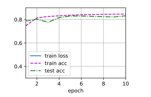
def train_ch3(net,train_iter,test_iter,loss,num_epochs,updater):
animator = Animator(xlabel='epoch',xlim=[1,num_epochs],ylim=[0.3,0.9],
legend=['train loss','train acc','test acc'])
for epoch in range(num_epochs): # 变量num_epochs遍数据
train_metrics = train_epoch_ch3(net,train_iter,loss,updater) # 返回两个值,一个总损失、一个总正确率
test_acc = evaluate_accuracy(net, test_iter) # 测试数据集上评估精度,仅返回一个值,总正确率
animator.add(epoch+1,train_metrics+(test_acc,)) # train_metrics+(test_acc,) 仅将两个值的正确率相加,
train_loss, train_acc = train_metrics
# 小批量随即梯度下降来优化模型的损失函数
lr = 0.1
def updater(batch_size):
return d2l.sgd([w,b],lr,batch_size)
num_epochs = 10
train_ch3(net,train_iter,test_iter,cross_entropy,num_epochs,updater)
2.10 预测数据
def predict_ch3(net,test_iter,n=6):
    for X, y in test_iter:
        break # 仅拿出一批六个数据
    trues = d2l.get_fashion_mnist_labels(y)
    preds = d2l.get_fashion_mnist_labels(net(X).argmax(axis=1))
    titles = [true + '\n' + pred for true, pred in zip(trues,preds)]
    d2l.show_images(X[0:n].reshape((n,28,28)),1,n,titles=titles[0:n])

predict_ch3(net,test_iter)
3. Sofmax回归(使用框架)
① 通过深度学习框架的高级API能够使实现softmax回归变得更加容易。
import torch
from torch import nn
from d2l import torch as d2l

batch_size = 256
train_iter, test_iter = d2l.load_data_fashion_mnist(batch_size)

# Softmax回归的输出是一个全连接层
# PyTorch不会隐式地调整输入的形状
# 因此,我们定义了展平层(flatten)在线性层前调整网络输入的形状
net = nn.Sequential(nn.Flatten(),nn.Linear(784,10))

def init_weights(m):
    if type(m) == nn.Linear:
        nn.init.normal_(m.weight, std=0.01) # 方差为0.01

net.apply(init_weights)
print(net.apply(init_weights)) # net网络的参数用的是init_weights初始化参数

# 在交叉熵损失函数中传递未归一化的预测,并同时计算softmax及其对数
loss = nn.CrossEntropyLoss()
# 使用学习率为0.1的小批量随即梯度下降作为优化算法
trainer = torch.optim.SGD(net.parameters(),lr=0.1)

num_epochs = 10
d2l.train_ch3(net,train_iter,test_iter,loss,num_epochs,trainer)
解释pytorch 函数之 nn.Flatten() 详细解释
nn.Flatten() 是 PyTorch 中的一个层(layer),它的作用是将输入的张量展平(flatten)。展平操作是将多维的张量转换为一维张量。在深度学习中,尤其是在卷积神经网络(CNN)中,通常需要在卷积层之后将多维的特征图展平为一维向量,然后将其输入到全连接层(nn.Linear)中进行分类或回归任务。
nn.Flatten() 的使用
1. 基本功能
nn.Flatten() 将输入张量从指定的维度开始展平,通常是展平所有除了批次维度以外的维度。最常见的用法是将图像数据(通常是 4D 张量,形状为 (batch_size, channels, height, width))展平为一个二维张量(形状为 (batch_size, channels * height * width)),以便输入到全连接层中。
2. 函数签名
nn.Flatten(start_dim=1, end_dim=-1)
start_dim:指定展平开始的维度。默认为 1,表示从第一个维度(即channels)开始展平。如果你不想展平批量维度(通常是第 0 维),可以保持这个值为 1。end_dim:指定展平结束的维度,默认为-1,表示一直展平到最后一个维度。
3. 具体示例
示例 1:简单的展平操作
假设我们有一个形状为 (batch_size, channels, height, width) 的图像数据,例如来自 CIFAR-10 数据集(每张图片为 32x32 像素,RGB 图像具有 3 个通道)。
import torch
from torch import nn

# 创建一个形状为 (batch_size, channels, height, width) 的输入张量
x = torch.randn(64, 3, 28, 28)  # batch_size=64, channels=3, height=28, width=28

# 使用 nn.Flatten 展平张量
flatten = nn.Flatten()
x_flat = flatten(x)

# 查看展平后的形状
print(x_flat.shape)  # 输出: torch.Size([64, 2352])
- 原始张量
x的形状是(64, 3, 28, 28),表示有 64 张图像,每张图像有 3 个通道(RGB),大小为 28x28 像素。 - 展平后的张量
x_flat的形状是(64, 2352),每张图像被展平为一个长度为 2352 的一维向量(3 * 28 * 28 = 2352)。
示例 2:指定 start_dim 和 end_dim
假设你有一个更复杂的多维张量,且你希望从某个特定维度开始展平。
# 创建一个形状为 (batch_size, channels, height, width, extra_dim) 的输入张量
x = torch.randn(64, 3, 28, 28, 2)  # batch_size=64, channels=3, height=28, width=28, extra_dim=2

# 使用 nn.Flatten 从第 1 维开始展平
flatten = nn.Flatten(start_dim=1)
x_flat = flatten(x)

# 查看展平后的形状
print(x_flat.shape)  # 输出: torch.Size([64, 2352, 2])
- 这里的原始张量
x具有形状(64, 3, 28, 28, 2),其中extra_dim=2是额外的维度。 - 使用
nn.Flatten(start_dim=1)将从第 1 维开始展平,这意味着channels,height,width, 和extra_dim维度都会被展平为一个大的一维向量。所以输出的形状是(64, 2352, 2),每个图像的数据被展平后,输出的每个样本是一个 2D 张量,其中第二维表示每个展平后的数据向量。
示例 3:展平到指定维度
如果你希望展平从某个维度到某个维度,例如从 height 到 width 之间的所有维度,你可以使用 end_dim 来指定展平的结束位置。
# 创建一个形状为 (batch_size, channels, height, width) 的输入张量
x = torch.randn(64, 3, 28, 28)  # batch_size=64, channels=3, height=28, width=28

# 使用 nn.Flatten 展平从第 2 维到第 3 维
flatten = nn.Flatten(start_dim=2, end_dim=3)
x_flat = flatten(x)

# 查看展平后的形状
print(x_flat.shape)  # 输出: torch.Size([64, 3, 784])
- 这里,
start_dim=2和end_dim=3表示从height(第 2 维)到width(第 3 维)之间的维度会被展平。channels(第 1 维)不会被展平。 - 结果是每个样本的形状从
(3, 28, 28)转变为(3, 784),每张图像的 28x28 的像素被展平成了一个长度为 784 的向量。
4. 应用场景
-
卷积神经网络(CNN):在卷积层之后,通常需要将卷积的输出展平为一维向量,以便传递到全连接层(
nn.Linear)中进行分类或回归任务。例如,卷积层通常会生成一个形状为(batch_size, channels, height, width)的张量,而全连接层通常期望输入是一个一维向量。因此,nn.Flatten()就是将这种多维张量展平为一维向量的常用工具。 -
多维数据展平:除了处理图像数据,
nn.Flatten()也可以用于处理任何形状的多维数据,在深度学习模型中展平数据以便进行后续的处理。
5. 总结
nn.Flatten()是一个非常简单但是强大的工具,用于将多维数据展平成一维张量,通常用于连接卷积层和全连接层。- 它可以通过
start_dim和end_dim参数控制从哪个维度开始展平,通常你会从start_dim=1开始展平,保留批量维度(第 0 维)。 - 它是深度学习中常用的数据预处理步骤之一,尤其在处理图像和卷积神经网络时。
解释pytorch 函数之nn.Linear() 详解
nn.Linear() 是 PyTorch 中用于定义 全连接层(fully connected layer)的一个类。它是神经网络中最常用的一种层,主要用于实现输入和输出的线性变换。每个全连接层由一个 权重矩阵 和一个 偏置向量 组成,用于对输入数据进行线性变换。通常在每个全连接层之后会应用一个非线性激活函数(如 ReLU、Sigmoid 或 Tanh)来引入非线性变换。
1. 函数签名
class torch.nn.Linear(in_features, out_features, bias=True)
in_features:输入的特征数,即输入张量的最后一个维度的大小。对于图像数据,它通常是展平后的像素数。out_features:输出的特征数,即该层输出张量的最后一个维度的大小。通常是网络的输出维度或下一层的输入维度。bias:是否使用偏置项,默认为True,即该层会有一个偏置项。如果设置为False,则不使用偏置项。
2. 功能和工作原理
nn.Linear() 定义了一个线性变换层,其实现是对输入张量 x 进行如下操作:
output=xWT+b\text{output} = xW^T + boutput=xWT+b
其中:
- xxx 是输入张量,大小为 [batch_size,in_features][batch\_size, in\_features][batch_size,in_features]。
- WWW 是权重矩阵,大小为 [out_features,in_features][out\_features, in\_features][out_features,in_features],这个矩阵会被训练。
- bbb 是偏置向量,大小为 [out_features][out\_features][out_features],也会被训练。
3. 计算过程
假设有一个批量大小为 batch_size 的输入张量 x,其形状为 (batch_size, in_features),nn.Linear(in_features, out_features) 会执行以下操作:
- 权重矩阵
W形状为(out_features, in_features)。 - 偏置向量
b形状为(out_features)(默认使用)。 - 输出张量的形状为
(batch_size, out_features)。
每个输出元素是由输入张量的每个元素与权重矩阵的对应元素进行加权求和,再加上偏置项。
4. 例子
4.1 简单示例:线性层
import torch
from torch import nn

# 输入特征数 (in_features) = 2, 输出特征数 (out_features) = 3
linear_layer = nn.Linear(2, 3)

# 创建一个形状为 (batch_size, in_features) 的输入张量
x = torch.randn(4, 2)  # batch_size=4, in_features=2

# 通过线性层
y = linear_layer(x)

# 打印输出的形状
print(y.shape)  # 输出: torch.Size([4, 3])
- 输入张量
x形状为(4, 2),表示批量大小为 4,每个样本有 2 个特征。 - 线性层 的输出张量
y形状为(4, 3),表示每个样本有 3 个输出特征。 - 内部,
nn.Linear(2, 3)自动初始化了权重矩阵W和偏置向量b,并将其用于计算输出。
4.2 权重初始化
# 打印线性层的权重和偏置
print("Weight matrix:")
print(linear_layer.weight)  # 权重矩阵 W,形状: [3, 2]

print("\nBias vector:")
print(linear_layer.bias)  # 偏置向量 b,形状: [3]
linear_layer.weight:这是权重矩阵,形状为[out_features, in_features],在本例中是[3, 2],表示输出特征数为 3,输入特征数为 2。linear_layer.bias:这是偏置向量,形状为[out_features],在本例中是[3],表示有 3 个输出特征,每个输出特征对应一个偏置。
4.3 计算过程
对于 x = [[x1, x2], [x3, x4], [x5, x6], [x7, x8]],如果线性层的权重矩阵 W 和偏置向量 b 已初始化,那么输出 y 将通过以下公式计算:
yi=W⋅xi+b y_i = W \cdot x_i + b yi=W⋅xi+b
- 对于每个样本 xix_ixi,计算对应的输出特征向量 yiy_iyi。
- 权重矩阵和偏置项是会在训练过程中更新的。
5. 实际应用
nn.Linear() 在以下场景中有广泛应用:
- 全连接层:将网络的前一层输出展平并传递到下一层。
- 多分类任务:在分类任务中,输出层通常是
nn.Linear(),它的输出维度对应于类别数。 - 回归任务:在回归任务中,输出层也可以是
nn.Linear(),它的输出通常是一个连续值。 - 神经网络中的多层感知器(MLP):全连接层是构建多层感知器的核心部分。
6. 训练与反向传播
在神经网络训练过程中,nn.Linear() 的权重和偏置会通过反向传播算法进行更新。对于每个训练样本,网络会计算误差(损失),然后通过反向传播来更新网络中的权重和偏置,从而减少误差并提高模型的准确性。
7. 总结
nn.Linear()是一个基本的神经网络层,用于实现输入和输出的线性变换。- 它包含一个权重矩阵和一个偏置向量,权重和偏置会在训练过程中进行优化。
- 在多层感知器(MLP)或深度学习模型中,
nn.Linear()是最常用的层之一。 - 典型的用法是将图像或其他数据展平并通过全连接层进行进一步处理,特别是在卷积神经网络(CNN)中。
通过理解 nn.Linear(),你可以更好地设计和实现神经网络模型,特别是处理高维数据时的输入和输出变换。
解释pytorch 函数之nn.Sequential() 详解
nn.Sequential() 是 PyTorch 中的一个容器类,用于按顺序组织神经网络的各个层。它允许用户将多个层(如卷积层、线性层、激活函数等)按顺序组合在一起,从而简化网络结构的定义和管理。
1. 函数签名
class torch.nn.Sequential(*args)
*args:Sequential类接受一个可变数量的层作为输入,层会按照传入的顺序被连接和执行。每一层的输出会作为下一层的输入。
2. 功能和工作原理
nn.Sequential() 的主要功能是将多个层按顺序连接在一起,并创建一个新的模块。Sequential 类会自动将前一层的输出传递到下一层。这使得定义简单的顺序模型变得非常容易,尤其是在模型层数较多时。
import torch
from torch import nn

# 使用 nn.Sequential 定义一个顺序模型
model = nn.Sequential(
    nn.Linear(784, 256),     # 第 1 层:线性变换
    nn.ReLU(),               # 第 2 层:ReLU 激活函数
    nn.Linear(256, 10)       # 第 3 层:线性变换
)
在上面的例子中,nn.Sequential 将三个层(nn.Linear 和 nn.ReLU)组合在一起,创建了一个顺序的网络结构。每一层会依次执行,数据会按顺序流经每一层。
3. 组件分析
3.1 每一层的顺序执行
在 nn.Sequential() 中,层按照定义的顺序逐个执行。也就是说,输入数据先经过第一个层(例如线性层),然后其输出作为下一个层的输入,依此类推。
例如,考虑下面的顺序网络:
model = nn.Sequential(
    nn.Conv2d(1, 32, kernel_size=3, padding=1),
    nn.ReLU(),
    nn.MaxPool2d(kernel_size=2, stride=2),
    nn.Conv2d(32, 64, kernel_size=3, padding=1),
    nn.ReLU(),
    nn.MaxPool2d(kernel_size=2, stride=2)
)
- 输入首先经过
Conv2d(1, 32, kernel_size=3, padding=1),该层将 1 个输入通道(灰度图像)转换为 32 个输出通道。 - 接着通过
ReLU()激活函数,使得网络具有非线性。 - 然后通过
MaxPool2d(kernel_size=2, stride=2)池化层,减小特征图的空间维度。 - 接下来的过程类似,经过第二个卷积层、激活函数和池化层。
3.2 层类型
nn.Sequential() 可以包含各种类型的层,包括但不限于:
- 线性层:
nn.Linear - 卷积层:
nn.Conv2d,nn.Conv1d - 池化层:
nn.MaxPool2d,nn.AvgPool2d - 激活函数:
nn.ReLU,nn.Sigmoid,nn.Tanh - 批量归一化层:
nn.BatchNorm2d,nn.BatchNorm1d - 丢弃层:
nn.Dropout
所有这些层都会按顺序连接,层的输出会作为下一个层的输入。
4. 使用 nn.Sequential() 组织模型
4.1 简单的前馈神经网络
假设你想实现一个简单的多层感知器(MLP),它有两个线性层和一个激活函数(ReLU)。你可以使用 nn.Sequential() 来定义模型:
model = nn.Sequential(
    nn.Linear(784, 256),   # 第 1 层:线性变换,输入特征 784,输出特征 256
    nn.ReLU(),             # 第 2 层:ReLU 激活函数
    nn.Linear(256, 10)     # 第 3 层:线性变换,输入特征 256,输出特征 10(对应 10 类)
)
这个模型有 3 层:第一层将输入的 784 维向量映射到 256 维,第二层是 ReLU 激活函数,第三层将 256 维向量映射到 10 维输出(对应于 10 类分类任务)。
4.2 更复杂的模型
假设你要构建一个包含卷积层、池化层、全连接层的卷积神经网络(CNN):
model = nn.Sequential(
    nn.Conv2d(1, 32, kernel_size=3, padding=1),   # 输入 1 个通道,输出 32 个通道
    nn.ReLU(),
    nn.MaxPool2d(kernel_size=2, stride=2),        # 池化,缩小尺寸
    nn.Conv2d(32, 64, kernel_size=3, padding=1),  # 输入 32 个通道,输出 64 个通道
    nn.ReLU(),
    nn.MaxPool2d(kernel_size=2, stride=2),        # 池化,缩小尺寸
    nn.Flatten(),                                 # 展平图像数据
    nn.Linear(64 * 7 * 7, 10)                     # 全连接层,输出 10 类
)
在这个模型中,数据从卷积层经过池化层、激活函数、再次经过卷积池化,最后被展平并传入一个全连接层进行分类。
5. 为什么使用 nn.Sequential()
- 简化代码:
nn.Sequential()可以大大简化模型的定义过程,特别是对于只包含顺序连接层的模型。在很多情况下,模型的每一层都是线性的,层与层之间没有复杂的连接(例如跳跃连接)。 - 代码清晰:通过按顺序定义网络结构,代码更加简洁易懂,尤其在构建较简单的模型时非常有用。
6. nn.Sequential() 的局限性
尽管 nn.Sequential() 使用起来非常简便,但它也有一定的局限性:
- 不支持跳跃连接:如果需要在网络中使用跳跃连接(如 ResNet 中的残差连接),
nn.Sequential()就不太适用了。在这种情况下,你需要显式地定义网络的前向传播(forward())函数。 - 灵活性较差:当网络中的层需要复杂的逻辑控制(如条件语句、不同分支的计算等)时,
nn.Sequential()无法满足需求。
如果需要更多的灵活性,可以通过自定义 nn.Module 类,并在 forward() 方法中实现更复杂的前向传播逻辑。
7. 总结
nn.Sequential()是一个简单而有效的容器,用于按顺序连接多个神经网络层。- 它能够简化模型的定义,特别适用于那些层与层之间顺序连接的简单网络。
- 适用于大多数常见的前馈网络结构,但在需要更高灵活性时,建议使用自定义的
nn.Module类。
通过合理使用 nn.Sequential(),你可以快速构建许多常见的神经网络架构,而无需编写繁琐的代码。


 964
964

 被折叠的 条评论
为什么被折叠?
被折叠的 条评论
为什么被折叠?
 到【灌水乐园】发言


