


英文是纯手打的!论文原文的summarizing and paraphrasing。可能会出现难以避免的拼写错误和语法错误,若有发现欢迎评论指正!文章偏向于笔记,谨慎食用
目录
2.3. Properties of Effective Receptive Fields
2.3.1. The simplest case: a stack of convolutional layers of weights all equal to one
2.3.4. Nonlinear activation functions
2.3.5. Dropout, Subsampling, Dilated Convolution and Skip-Connections
2.4.1. Verifying theoretical results
2.4.2. How the ERF evolves during training
2.5. Reduce the Gaussian Damage
1. 心得
(1)这篇文章是16年的让25年的我像个joker
2. 论文逐段精读
2.1. Abstract
①They aim to research receptive fields (RF) of units
②Effective receptive field (ERF) is part of theoretical receptive field (TRF)
2.2. Introduction
①Not all the pixels in the TRF contribute the same
②ERF distributes as a Gaussian
③⭐Compared with large kernel conv, the deep net with small kernel might indicates a bad initialization bias on initial small ERF
2.3. Properties of Effective Receptive Fields
①Pixel index:
②Image center:
③Pixel in the -th conv layer:
, where
is the input
④Output:
⑤Task: measure how contribute to
by
⑥Back propagation function: where
denotes the loss
⑦To get the answer, they define error gradient and
for all
and
, then
(虽然这个等式代入⑤的确成立吧,但是它理由是啥啊??就直接随便定义上面俩等于1和0吗)
2.3.1. The simplest case: a stack of convolutional layers of weights all equal to one
①Consider conv layers with kernel size
, stride
, channel
, no linear function
② is the gradient on the
-th layer,
③Desired result:
④They define initial gradient signal and kernel
:
where
⑤Gradient signal on each input pixel:
⑥Calculate these conv by Discrete Time Fourier Transform:
⑦Fourier transform is
⑧Inverse Fourier transform:
2.3.2. Random weights
①There is pixel indices shifting:
②Known , there is:
③Passing a kernel with full 1's:
2.3.3. Non-uniform kernels
①Weights are normalized:
②So:
and the mean and variance of this Gaussian:
③A standard deviation as the radius of ERF:
where 's are i.i.d. multinomial variables distributed according to
's, e.g.
④Compared with TRF, ERF shrinks ar a rate of
2.3.4. Nonlinear activation functions
①For non linear activation function and a conv, there is:
where is the gradient of the activation function for pixel
at layer
②If gradients are independent from the weights and
in the upper layer, the variance can be simplified by:
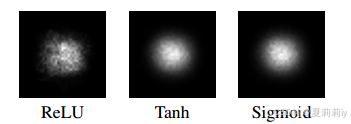
just for ReLU, it's hard for analysing Sigmoid and Tanh
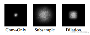
2.3.5. Dropout, Subsampling, Dilated Convolution and Skip-Connections
①Dropout won't change the shape of ERF
②Subsampling and dilated convolutions can increase the erea of ERF
2.4. Experiments
2.4.1. Verifying theoretical results
①Vis of ERF:
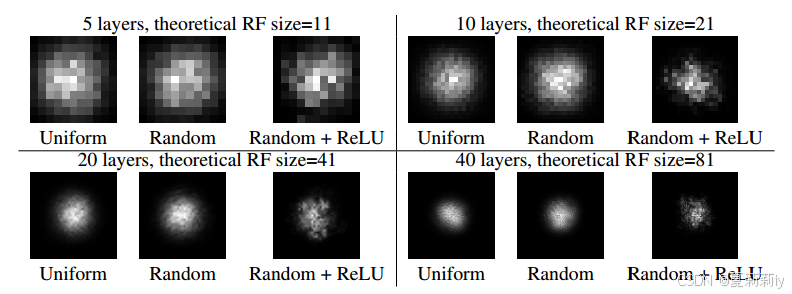
where non linear function weaken the Gaussian distribution, and kernel size there is 3 × 3, weights of kernal are all 1 in Uniform and are random in Random
②Though non linear function corrupt Gaussian distribution, average of 100 running times may change this situation:
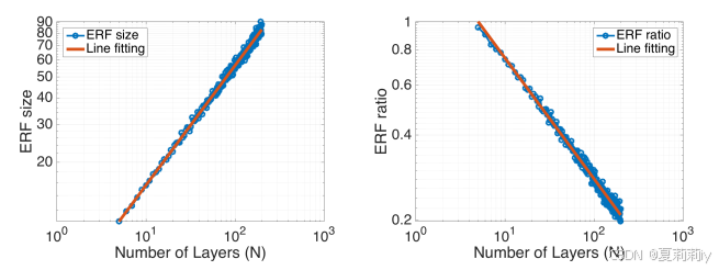
③Absolute growth (left) and relative shrink (right) for ERF:
④Subsample and dilation expand the ERF:
2.4.2. How the ERF evolves during training
①ERF before and after training on CIFAR-10 classification and CamVid semantic segmentation:
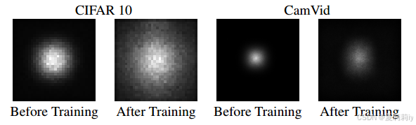
and TRF remains the same
2.5. Reduce the Gaussian Damage
①Assign less weight on the center of kernel but higher on the outside
2.6. Discussion
①一些畅想,也就不说了
2.7. Conclusion
~
asymptotically adv.渐近地
3. Reference
Luo, W. et al. (2016) Understanding the effective receptive field in deep convolutional neural networks, NeurIPS. Red Hook, NY, USA.


 6267
6267

 被折叠的 条评论
为什么被折叠?
被折叠的 条评论
为什么被折叠?
 到【灌水乐园】发言


