


 文章介绍了BitNet技术,一种在大型语言模型中使用1-bit量化的方法,包括absmax量化、权重的二值化和直通估计策略。通过分组处理,它实现了高效的计算并保持量化后的方差。BitLinear类展示了如何在PyTorch中实现这一技术。
输入数据
-
模型使用absmax 量化方法进行b比特量化,将输入量化到 [ − Q b , Q b ] ( Q b = 2 b − 1 ) \left[-Q_{b},Q_{b}\right](Q_{b}=2^{b-1}) [−Qb,Qb](Qb=2b−1)
x ~ = Q u a n t ( x ) = C l i p ( x × Q b γ , − Q b + ϵ , Q b − ϵ ) , Clip ( x , a , b ) = max ( a , min ( b , x ) ) , γ = ∣ ∣ x ∣ ∣ ∞ , \widetilde{x}=\mathrm{Quant}(x)=\mathrm{Clip}(x\times\frac{Q_b}{\gamma},-Q_b+\epsilon,Q_b-\epsilon),\\ \operatorname{Clip}(x,a,b)=\max(a,\min(b,x)),\quad\gamma=||x||_\infty, x =Quant(x)=Clip(x×γQb,−Qb+ϵ,Qb−ϵ),Clip(x,a,b)=max(a,min(b,x)),γ=∣∣x∣∣∞, -
其中 ε 是一个小的浮点数,可防止在执行截断时溢出。
// https://github.com/kyegomez/BitNet/blob/main/bitnet/bitbnet_b158.py
def absmean_quantize_weights(weights):
    """
    Quantizes the weights to -1, 0, or +1 using an absmean quantization function.

    Parameters:
    - weights (Tensor): The weights of a neural network layer.

    Returns:
    - Tensor: The quantized weights.
    """
    # Calculate the average absolute value (γ) of the weights
    gamma = torch.mean(torch.abs(weights))

    # Scale weights by γ and round to the nearest integer among {-1, 0, +1}
    quantized_weights = torch.clamp(torch.round(weights / gamma), min=-1, max=1)

    return quantized_weights
权重
- 权重 W 的二值化可以公式化为:
α = 1 n m ∑ i j W i j W ~ = S i g n ( W − α ) , Sign ( W i j ) = { + 1 , if W i j > 0 , − 1 , if W i j ≤ 0 , \\ \alpha=\frac1{nm}\sum_{ij}W_{ij} \\ \widetilde{W}=\mathrm{Sign}(W-\alpha),\\ \left.\operatorname{Sign}(W_{ij})=\left\{\begin{array}{ll}+1,&\quad\text{if}W_{ij}>0,\\-1,&\quad\text{if}W_{ij}\leq0,\end{array}\right.\right. α=nm1ij∑WijW =Sign(W−α),Sign(Wij)={+1,−1,ifWij>0,ifWij≤0,
矩阵乘法
- 使用上述量化方程,矩阵乘法可以写成:
y = W ~ x ~ y=\widetilde W\widetilde{x} y=W x
- 为了保持量化后的方差,我们在激活量化之前引入了一个 LayerNorm函数。这样,输出 y 的方差就估计为 1
y
=
W
~
x
~
=
W
~
Quant
(
LN
(
x
)
)
×
β
γ
Q
b
y=\widetilde{W}\widetilde{x}=\widetilde{W}\text{Quant}(\text{LN}(x))\times\frac{\beta\gamma}{Q_b}
y=W
x
=W
Quant(LN(x))×Qbβγ
L
N
(
x
)
=
x
−
E
(
x
)
V
a
r
(
x
)
+
ϵ
,
β
=
1
n
m
∥
W
∥
1
\mathrm{LN}(x)=\frac{x-E(x)}{\sqrt{\mathrm{Var}(x)+\epsilon}},\quad\beta=\frac1{nm}\|W\|_1
LN(x)=Var(x)+ϵx−E(x),β=nm1∥W∥1

// https://github.com/kyegomez/BitNet/blob/main/bitnet/bitlinear.py
import torch
from torch import Tensor, nn
class BitLinear(nn.Linear):
"""
BitLinear is a custom linear layer that performs binarization of weights and quantization of activations
in a group-wise manner.
Args:
in_features (int): Number of input features.
out_features (int): Number of output features.
bias (bool, optional): If set to False, the layer will not learn an additive bias. Default is True.
num_groups (int, optional): Number of groups to divide the weights and activations into. Default is 1.
"""
def __init__(
self,
in_features: int,
out_features: int,
bias: bool = True,
num_groups: int = 1,
b: int = 8,
):
super().__init__(in_features, out_features, bias)
self.in_features = in_features
self.out_features = out_features
self.b = b
self.num_groups = num_groups
self.eps = 1e-5
self.norm = nn.LayerNorm(in_features)
def ste(self, x):
"""
Applies the sign function for binarization and uses Straight-Through Estimator (STE) during backward pass.
Args:
x (Tensor): Input tensor.
Returns:
Tensor: Binarized tensor.
"""
binarized_x = torch.sign(x)
binarized_x = (binarized_x - x).detach() + x
return binarized_x
def binarize_weights_groupwise(self):
"""
Binarizes the weights of the layer in a group-wise manner using STE.
Returns:
Tensor: Binarized weights tensor.
"""
group_size = self.weight.shape[0] // self.num_groups
binarized_weights = torch.zeros_like(self.weight)
for g in range(self.num_groups):
start_idx = g * group_size
end_idx = (g + 1) * group_size
weight_group = self.weight[start_idx:end_idx]
alpha_g = weight_group.mean()
binarized_weights[start_idx:end_idx] = self.ste(weight_group - alpha_g)
return binarized_weights
def quantize_activations_groupwise(self, x):
"""
Quantizes the activations of the layer in a group-wise manner.
Args:
x (Tensor): Input tensor.
b (int, optional): Number of bits for quantization. Default is 8.
Returns:
Tensor: Quantized activations tensor.
"""
Q_b = 2 ** (self.b - 1)
group_size = x.shape[0] // self.num_groups
quantized_x = torch.zeros_like(x)
for g in range(self.num_groups):
start_idx = g * group_size
end_idx = (g + 1) * group_size
activation_group = x[start_idx:end_idx]
gamma_g = activation_group.abs().max()
quantized_x[start_idx:end_idx] = torch.clamp(
activation_group * Q_b / (gamma_g + self.eps),
-Q_b + self.eps,
Q_b - self.eps,
)
return quantized_x
def dequantize_activations_groupwise(self, x):
"""
Dequantizes the activations of the layer in a group-wise manner.
Args:
x (Tensor): Quantized input tensor.
b (int, optional): Number of bits used during the quantization. Default is 8.
Returns:
Tensor: Dequantized activations tensor.
"""
Q_b = 2 ** (self.b - 1)
dequantized_x = torch.zeros_like(x)
for g in range(self.num_groups):
start_idx = g * x.shape[0] // self.num_groups
end_idx = (g + 1) * x.shape[0] // self.num_groups
quantized_group = x[start_idx:end_idx]
gamma_g = quantized_group.abs().max()
dequantized_x[start_idx:end_idx] = quantized_group * gamma_g / Q_b
return dequantized_x
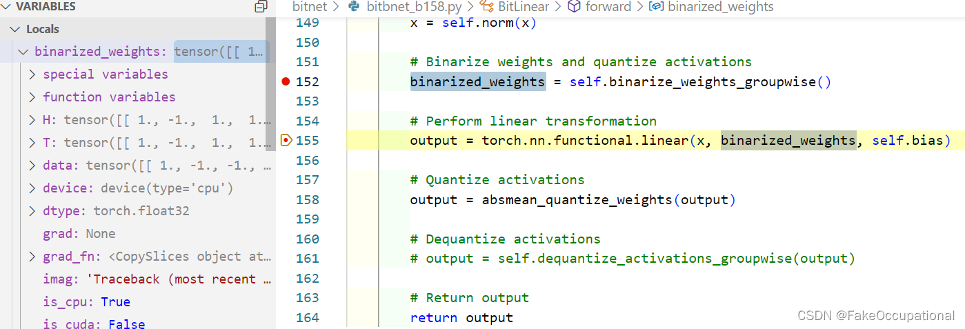
def forward(self, x: Tensor) -> Tensor:
"""
Forward pass of the BitLinear layer.
Args:
x (Tensor): Input tensor.
Returns:
Tensor: Output tensor.
"""
# Normalize input
x = self.norm(x)
# Binarize weights and quantize activations
binarized_weights = self.binarize_weights_groupwise()
# Perform linear transformation
output = torch.nn.functional.linear(x, binarized_weights, self.bias)
# Quantize activations
output = self.quantize_activations_groupwise(output)
# Dequantize activations
output = self.dequantize_activations_groupwise(output)
# Return output
return output
# Example usage
bitlinear = BitLinear(10, 5, num_groups=2, b=8)
input_tensor = torch.randn(5, 10) # Example input tensor
output = bitlinear(input_tensor)
print(output) # Example output tensor


 226
226

 被折叠的 条评论
为什么被折叠?
被折叠的 条评论
为什么被折叠?
 到【灌水乐园】发言


