保姆级教程【车道线检测】，跟着一步一步来，小学生都可以学会吧

粉丝福利：

开始之前，迪迦给大家准备的250G人工智能学习资料礼包（内含：两大Pytorch、TensorFlow实战框架视频、图像识别、OpenCV、计算机视觉、深度学习与神经网络等等等视频、代码、PPT以及深度学习书籍）

只需要你点个关注，然后扫码添加助手小姐姐VX即可无套路领取！

  扫码添加即可 

项目描述：

使用openCV设计算法处理车辆前置摄像头录下的视频，检测车辆前方的车道，并计算车道曲率

项目代码地址：https://github.com/yang1688899/CarND-Advanced-Lane-Lines

实现步骤：

• 使用提供的一组棋盘格图片计算相机校正矩阵(camera calibration matrix)和失真系数(distortion coefficients).
• 校正图片
• 使用梯度阈值(gradient threshold)，颜色阈值(color threshold)等处理图片得到清晰捕捉车道线的二进制图(binary image).
• 使用透视变换(perspective transform)得到二进制图(binary image)的鸟瞰图(birds-eye view).
• 检测属于车道线的像素并用它来测出车道边界.
• 计算车道曲率及车辆相对车道中央的位置.
• 处理图片展示车道区域，及车道的曲率和车辆位置.

相机校正(Camera Calibration)

这里会使用opencv提供的方法通过棋盘格图片组计算相机校正矩阵(camera calibration matrix)和失真系数(distortion coefficients)。首先要得到棋盘格内角的世界坐标"object points"和对应图片坐标"image point"。假设棋盘格内角世界坐标的z轴为0，棋盘在(x,y)面上，则对于每张棋盘格图片组的图片而言，对应"object points"都是一样的。而通过使用openCv的cv2.findChessboardCorners()，传入棋盘格的灰度(grayscale)图片和横纵内角点个数就可得到图片内角的"image point"。

def get_obj_img_points(images,grid=(9,6)):
    object_points=[]
    img_points = []
    for img in images:
        #生成object points
        object_point = np.zeros( (grid[0]*grid[1],3),np.float32 )
        object_point[:,:2]= np.mgrid[0:grid[0],0:grid[1]].T.reshape(-1,2)
        #得到灰度图片
        gray = cv2.cvtColor(img,cv2.COLOR_BGR2GRAY)
        #得到图片的image points
        ret, corners = cv2.findChessboardCorners(gray, grid, None)
        if ret:
            object_points.append(object_point)
            img_points.append(corners)
    return object_points,img_points

然后使用上方法得到的object_points and img_points 传入cv2.calibrateCamera() 方法中就可以计算出相机校正矩阵(camera calibration matrix)和失真系数(distortion coefficients)，再使用 cv2.undistort()方法就可得到校正图片。

def cal_undistort(img, objpoints, imgpoints):
    ret, mtx, dist, rvecs, tvecs = cv2.calibrateCamera(objpoints, imgpoints, img.shape[1::-1], None, None)
    dst = cv2.undistort(img, mtx, dist, None, mtx)
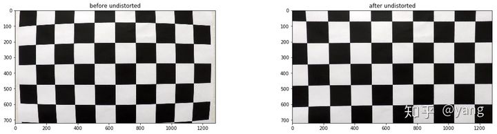
    return dst

以下为其中一张棋盘格图片校正前后对比：

校正测试图片

代码如下：

#获取棋盘格图片
cal_imgs = utils.get_images_by_dir('camera_cal')
#计算object_points,img_points
object_points,img_points = utils.calibrate(cal_imgs,grid=(9,6))
#获取测试图片
test_imgs = utils.get_images_by_dir('test_images')

#校正测试图片
undistorted = []
for img in test_imgs:
    img = utils.cal_undistort(img,object_points,img_points)
    undistorted.append(img)

测试图片校正前后对比：

阈值过滤(thresholding)

这里会使用梯度阈值(gradient threshold)，颜色阈值(color threshold)等来处理校正后的图片，捕获车道线所在位置的像素。(这里的梯度指的是颜色变化的梯度)

以下方法通过"cv2.Sobel()"方法计算x轴方向或y轴方向的颜色变化梯度导数，并以此进行阈值过滤(thresholding),得到二进制图(binary image)：

def abs_sobel_thresh(img, orient='x', thresh_min=0, thresh_max=255):
    #装换为灰度图片
    gray = cv2.cvtColor(img, cv2.COLOR_RGB2GRAY)
    #使用cv2.Sobel()计算计算x方向或y方向的导数
    if orient == 'x':
        abs_sobel = np.absolute(cv2.Sobel(gray, cv2.CV_64F, 1, 0))
    if orient == 'y':
        abs_sobel = np.absolute(cv2.Sobel(gray, cv2.CV_64F, 0, 1))
    #阈值过滤
    scaled_sobel = np.uint8(255*abs_sobel/np.max(abs_sobel))
    binary_output = np.zeros_like(scaled_sobel)
    binary_output[(scaled_sobel >= thresh_min) & (scaled_sobel <= thresh_max)] = 1

    return binary_output

通过测试发现使用x轴方向阈值在35到100区间过滤得出的二进制图可以捕捉较为清晰的车道线：

x_thresh = utils.abs_sobel_thresh(img, orient='x', thresh_min=35, thresh_max=100)

以下为使用上面方法应用测试图片的过滤前后对比图：

可以看到该方法的缺陷是在路面颜色相对较浅且车道线颜色为黄色时，无法捕捉到车道线（第三，第六，第七张图），但在其他情况车道线捕捉效果还是不错的。

接下来测试一下使用全局的颜色变化梯度来进行阈值过滤：

def mag_thresh(img, sobel_kernel=3, mag_thresh=(0, 255)):
    # Convert to grayscale
    gray = cv2.cvtColor(img, cv2.COLOR_RGB2GRAY)
    # Take both Sobel x and y gradients
    sobelx = cv2.Sobel(gray, cv2.CV_64F, 1, 0, ksize=sobel_kernel)
    sobely = cv2.Sobel(gray, cv2.CV_64F, 0, 1, ksize=sobel_kernel)
    # Calculate the gradient magnitude
    gradmag = np.sqrt(sobelx**2 + sobely**2)
    # Rescale to 8 bit
    scale_factor = np.max(gradmag)/255 
    gradmag = (gradmag/scale_factor).astype(np.uint8) 
    # Create a binary image of ones where threshold is met, zeros otherwise
    binary_output = np.zeros_like(gradmag)
    binary_output[(gradmag >= mag_thresh[0]) & (gradmag <= mag_thresh[1])] = 1

    # Return the binary image
    return binary_output
mag_thresh = utils.mag_thresh(img, sobel_kernel=9, mag_thresh=(50, 100))

结果仍然不理想(观察第三，第六，第七张图片)，原因是当路面颜色相对较浅且车道线颜色为黄色时，颜色变化梯度较小，想要把捕捉车道线需要把阈值下限调低，然而这样做同时还会捕获大量的噪音像素，效果会更差。

那么使用颜色阈值过滤呢？ 下面为使用hls颜色空间的s通道进行阈值过滤：

def hls_select(img,channel='s',thresh=(0, 255)):
    hls = cv2.cvtColor(img, cv2.COLOR_RGB2HLS)
    if channel=='h':
        channel = hls[:,:,0]
    elif channel=='l':
        channel=hls[:,:,1]
    else:
        channel=hls[:,:,2]
    binary_output = np.zeros_like(channel)
    binary_output[(channel > thresh[0]) & (channel <= thresh[1])] = 1
    return binary_output
s_thresh = utils.hls_select(img,channel='s',thresh=(180, 255))

可以看到在路面颜色相对较浅且车道线颜色为黄色的区域，车道线仍然被清晰的捕捉到了，然而在其他地方表现却不太理想(第四，第八张图片)

因此为了应对多变的路面情况，需要结合多种阈值过滤方法。

以下为最终的阈值过滤组合：

def thresholding(img):
    x_thresh = utils.abs_sobel_thresh(img, orient='x', thresh_min=10 ,thresh_max=230)
    mag_thresh = utils.mag_thresh(img, sobel_kernel=3, mag_thresh=(30, 150))
    dir_thresh = utils.dir_threshold(img, sobel_kernel=3, thresh=(0.7, 1.3))
    hls_thresh = utils.hls_select(img, thresh=(180, 255))
    lab_thresh = utils.lab_select(img, thresh=(155, 200))
    luv_thresh = utils.luv_select(img, thresh=(225, 255))
    #Thresholding combination
    threshholded = np.zeros_like(x_thresh)
    threshholded[((x_thresh == 1) & (mag_thresh == 1)) | ((dir_thresh == 1) & (hls_thresh == 1)) | (lab_thresh == 1) | (luv_thresh == 1)] = 1

    return threshholded

透视变换(perspective transform)

这里使用"cv2.getPerspectiveTransform()"来获取变形矩阵(tranform matrix)，把阈值过滤后的二进制图片变形为鸟撒视角。

以下为定义的源点（source points）和目标点（destination points）

Source Destination 585, 460320, 0203, 720320, 7201127, 720960, 720695, 460960, 0

定义方法获取变形矩阵和逆变形矩阵：

def get_M_Minv():
    src = np.float32([[(203, 720), (585, 460), (695, 460), (1127, 720)]])
    dst = np.float32([[(320, 720), (320, 0), (960, 0), (960, 720)]])
    M = cv2.getPerspectiveTransform(src, dst)
    Minv = cv2.getPerspectiveTransform(dst,src)
    return M,Minv

然后使用"cv2.warpPerspective()"传入相关值获得变形图片(wrapped image)

thresholded_wraped = cv2.warpPerspective(thresholded, M, img.shape[1::-1], flags=cv2.INTER_LINEAR)

以下为原图及变形后的效果：

以下为阈值过滤后二进制图变形后效果：

检测车道边界

上面的二进制图还存在一定的噪音像素，为了准确检测车道边界，首先要确定哪些像素是属于车道线的。

首先要定位车道线的基点(图片最下方车道出现的x轴坐标)，由于车道线在的像素都集中在x轴一定范围内，因此把图片一分为二，左右两边的在x轴上的像素分布峰值非常有可能就是车道线基点。

以下为测试片x轴的像素分布图：

定位基点后，再使用使用滑动窗多项式拟合(sliding window polynomial fitting)来获取车道边界。这里使用9个200px宽的滑动窗来定位一条车道线像素：

def find_line(binary_warped):
    # Take a histogram of the bottom half of the image
    histogram = np.sum(binary_warped[binary_warped.shape[0]//2:,:], axis=0)
    # Find the peak of the left and right halves of the histogram
    # These will be the starting point for the left and right lines
    midpoint = np.int(histogram.shape[0]/2)
    leftx_base = np.argmax(histogram[:midpoint])
    rightx_base = np.argmax(histogram[midpoint:]) + midpoint
    
    # Choose the number of sliding windows
    nwindows = 9
    # Set height of windows
    window_height = np.int(binary_warped.shape[0]/nwindows)
    # Identify the x and y positions of all nonzero pixels in the image
    nonzero = binary_warped.nonzero()
    nonzeroy = np.array(nonzero[0])
    nonzerox = np.array(nonzero[1])
    # Current positions to be updated for each window
    leftx_current = leftx_base
    rightx_current = rightx_base
    # Set the width of the windows +/- margin
    margin = 100
    # Set minimum number of pixels found to recenter window
    minpix = 50
    # Create empty lists to receive left and right lane pixel indices
    left_lane_inds = []
    right_lane_inds = []
    
    # Step through the windows one by one
    for window in range(nwindows):
        # Identify window boundaries in x and y (and right and left)
        win_y_low = binary_warped.shape[0] - (window+1)*window_height
        win_y_high = binary_warped.shape[0] - window*window_height
        win_xleft_low = leftx_current - margin
        win_xleft_high = leftx_current + margin
        win_xright_low = rightx_current - margin
        win_xright_high = rightx_current + margin
        # Identify the nonzero pixels in x and y within the window
        good_left_inds = ((nonzeroy >= win_y_low) & (nonzeroy < win_y_high) & 
        (nonzerox >= win_xleft_low) &  (nonzerox < win_xleft_high)).nonzero()[0]
        good_right_inds = ((nonzeroy >= win_y_low) & (nonzeroy < win_y_high) & 
        (nonzerox >= win_xright_low) &  (nonzerox < win_xright_high)).nonzero()[0]
        # Append these indices to the lists
        left_lane_inds.append(good_left_inds)
        right_lane_inds.append(good_right_inds)
        # If you found > minpix pixels, recenter next window on their mean position
        if len(good_left_inds) > minpix:
            leftx_current = np.int(np.mean(nonzerox[good_left_inds]))
        if len(good_right_inds) > minpix:        
            rightx_current = np.int(np.mean(nonzerox[good_right_inds]))
    
    # Concatenate the arrays of indices
    left_lane_inds = np.concatenate(left_lane_inds)
    right_lane_inds = np.concatenate(right_lane_inds)
    
    # Extract left and right line pixel positions
    leftx = nonzerox[left_lane_inds]
    lefty = nonzeroy[left_lane_inds] 
    rightx = nonzerox[right_lane_inds]
    righty = nonzeroy[right_lane_inds] 
    
    # Fit a second order polynomial to each
    left_fit = np.polyfit(lefty, leftx, 2)
    right_fit = np.polyfit(righty, rightx, 2)
    
    return left_fit, right_fit, left_lane_inds, right_lane_inds

以下为滑动窗多项式拟合(sliding window polynomial fitting)得到的结果：

计算车道曲率及车辆相对车道中心位置

利用检测车道得到的拟合值(find_line 返回的left_fit, right_fit)计算车道曲率，及车辆相对车道中心位置：

def calculate_curv_and_pos(binary_warped,left_fit, right_fit):
    # Define y-value where we want radius of curvature
    ploty = np.linspace(0, binary_warped.shape[0]-1, binary_warped.shape[0] )
    leftx = left_fit[0]*ploty**2 + left_fit[1]*ploty + left_fit[2]
    rightx = right_fit[0]*ploty**2 + right_fit[1]*ploty + right_fit[2]
    # Define conversions in x and y from pixels space to meters
    ym_per_pix = 30/720 # meters per pixel in y dimension
    xm_per_pix = 3.7/700 # meters per pixel in x dimension
    y_eval = np.max(ploty)
    # Fit new polynomials to x,y in world space
    left_fit_cr = np.polyfit(ploty*ym_per_pix, leftx*xm_per_pix, 2)
    right_fit_cr = np.polyfit(ploty*ym_per_pix, rightx*xm_per_pix, 2)
    # Calculate the new radii of curvature
    left_curverad = ((1 + (2*left_fit_cr[0]*y_eval*ym_per_pix + left_fit_cr[1])**2)**1.5) / np.absolute(2*left_fit_cr[0])
    right_curverad = ((1 + (2*right_fit_cr[0]*y_eval*ym_per_pix + right_fit_cr[1])**2)**1.5) / np.absolute(2*right_fit_cr[0])
    
    curvature = ((left_curverad + right_curverad) / 2)
    #print(curvature)
    lane_width = np.absolute(leftx[719] - rightx[719])
    lane_xm_per_pix = 3.7 / lane_width
    veh_pos = (((leftx[719] + rightx[719]) * lane_xm_per_pix) / 2.)
    cen_pos = ((binary_warped.shape[1] * lane_xm_per_pix) / 2.)
    distance_from_center = veh_pos - cen_pos
    return curvature,distance_from_center

处理原图，展示信息

使用逆变形矩阵把鸟瞰二进制图检测的车道镶嵌回原图，并高亮车道区域:

def draw_area(undist,binary_warped,Minv,left_fit, right_fit):
    # Generate x and y values for plotting
    ploty = np.linspace(0, binary_warped.shape[0]-1, binary_warped.shape[0] )
    left_fitx = left_fit[0]*ploty**2 + left_fit[1]*ploty + left_fit[2]
    right_fitx = right_fit[0]*ploty**2 + right_fit[1]*ploty + right_fit[2]
    # Create an image to draw the lines on
    warp_zero = np.zeros_like(binary_warped).astype(np.uint8)
    color_warp = np.dstack((warp_zero, warp_zero, warp_zero))
    
    # Recast the x and y points into usable format for cv2.fillPoly()
    pts_left = np.array([np.transpose(np.vstack([left_fitx, ploty]))])
    pts_right = np.array([np.flipud(np.transpose(np.vstack([right_fitx, ploty])))])
    pts = np.hstack((pts_left, pts_right))
    
    # Draw the lane onto the warped blank image
    cv2.fillPoly(color_warp, np.int_([pts]), (0,255, 0))
    
    # Warp the blank back to original image space using inverse perspective matrix (Minv)
    newwarp = cv2.warpPerspective(color_warp, Minv, (undist.shape[1], undist.shape[0])) 
    # Combine the result with the original image
    result = cv2.addWeighted(undist, 1, newwarp, 0.3, 0)
    return result

使用"cv2.putText()"方法处理原图展示车道曲率及车辆相对车道中心位置信息：

def draw_values(img, curvature, distance_from_center):
    font = cv2.FONT_HERSHEY_SIMPLEX
    radius_text = "Radius of Curvature: %sm" % (round(curvature))

    if distance_from_center > 0:
        pos_flag = 'right'
    else:
        pos_flag = 'left'

    cv2.putText(img, radius_text, (100, 100), font, 1, (255, 255, 255), 2)
    center_text = "Vehicle is %.3fm %s of center" % (abs(distance_from_center), pos_flag)
    cv2.putText(img, center_text, (100, 150), font, 1, (255, 255, 255), 2)
    return img

以下为测试图片处理后结果：

(ps：最近在重新看一些udacity上做的项目，就顺便整理下来写成文章分享一下，以后陆续还会写一些，谢谢关注)

原文链接：车道线检测 - 知乎