


 本文深入探讨了VC维数的概念及其在机器学习中的应用。主要内容包括VC维数的定义、感知机的VC维数、VC维数的物理直觉以及如何解释VC维数。通过这些内容,读者将了解到VC维数如何帮助评估学习算法的有效性和复杂性。
目录
Video1: Definition of VC Dimension
Recap: More on Growth Function
Video2: VC Dimension of Perceptrons
Video3: Physical Intuition of VC Dimension
Video4: Interpreting VC Dimension
VC Bound Rephrase: Penalty for Model Complexity
VC Bound Rephrase: Sample Complexity
Video1: Definition of VC Dimension
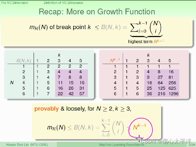
Recap: More on Growth Function
- 回顾之前的内容:
- 找到了growth function 的上限是 B(N, k)
- B(N, k) 的上限是
- 以上必须在 N ≧ 2 , k ≧ 3 的条件下才成立
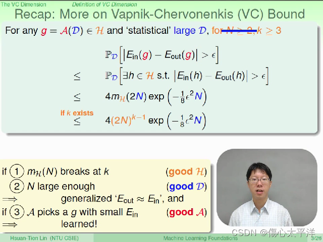
Recap: More on VC bound
- 回顾之前的内容:
- 找到坏事发生几率式子的上限
- 但前提是 N 够大,且具有 break point, k
- 只要演算法能够挑选到好的 g,则学习是可行的
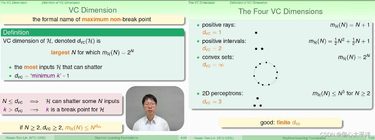
VC Dimension
- VC Dimension,
: Hypothesis 可以 shatter 的最大数据量
- 若
,则
- 一个好的 hypothesis set ,其 VC Dimension 必须是有限大小的
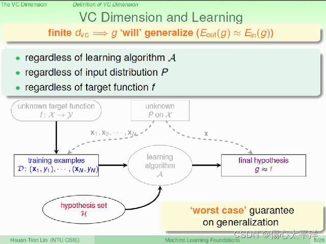
VC Dimension and Learning
- 只要VC Dimension 是有限的,则坏事发生的几率很小,我们可以准确估算模型的效果
- 即使在最坏的情况下,学习仍是可行的
- VC Dimension 与挑选 g 的演算法无关
- VC Dimension 与数据的分布 p 无关
- VC Dimension 与目标函数 f 无关
Video2: VC Dimension of Perceptrons
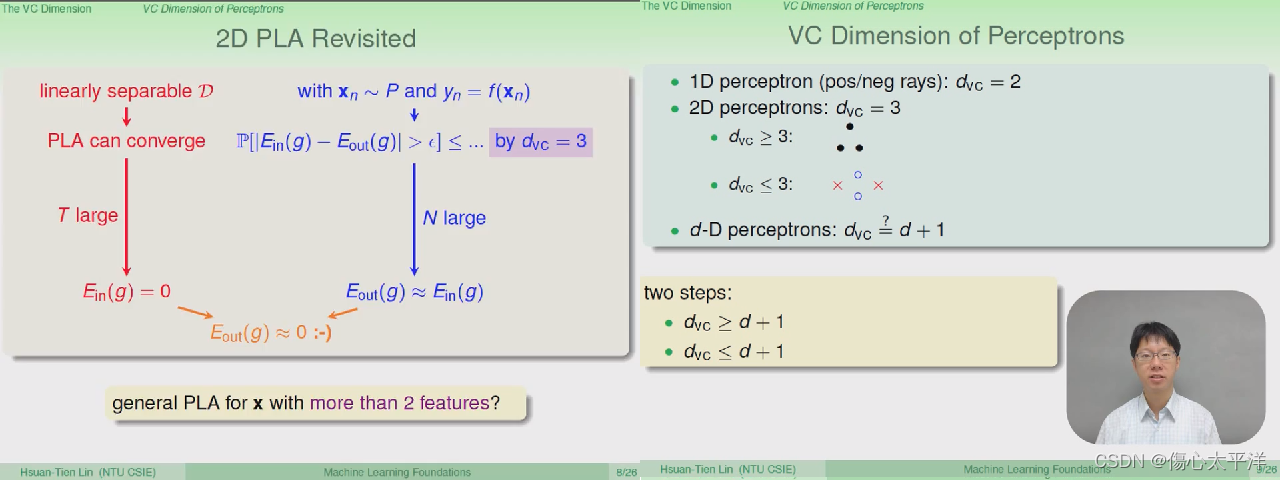
2D PLA Revisited
- 前面说明了
- 只要数据是线性可分,则在经过多次的迭代后,PLA 能够找到完美的分类线
- 只要 VC dimension 是有限的,且 N 够大,则验证结果会与实际结果差不多
- 如果是更高维度的 perceptron ?
- 1-D perceptron
- 证明的部份,可以先证明
,再证明
- 1-D perceptron
 证明(1)
证明(1)
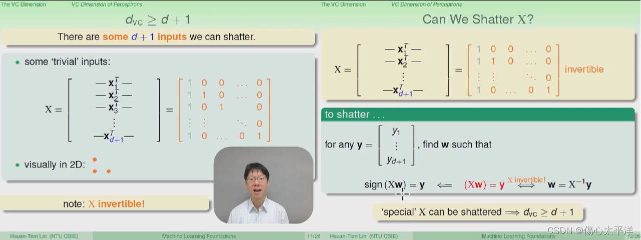
- 要证明
- 证明过程
- 使用了一组特殊的数据点: 原点 + 只有一个维度为 1 其余为 0 的共 d+1 个数据点
- 因为矩阵 x 是可逆的,所以任何 y 值都能找到相对应的 w
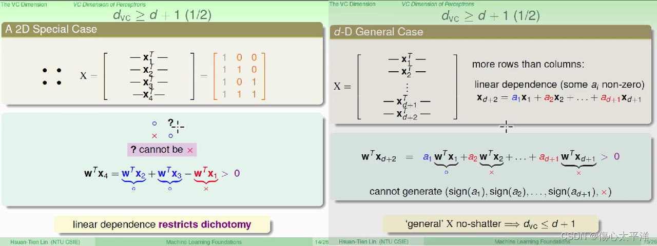
证明(2)
- 要证明
,只要找出一组 d+2 数据无法被 shatter 的例子即可
- 证明过程
- 使用了与证明(1)相同的数据点,但再加上一个数据点 (第 d+2 个点)
- 第 d+2 个点会发生线性相依,因此必定是由前面 d+1 个点的线性组合所构成
- 因此第 d+2 个点的分类结果,无法任意决定,所以无法 shatter d+2 个点
Video3: Physical Intuition of VC Dimension
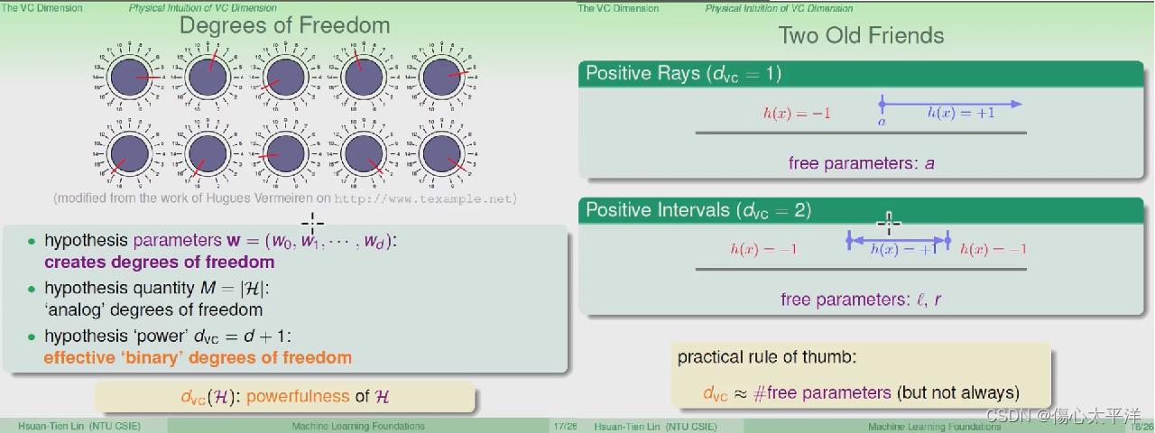
Degree of Freedom
- 如果把 Hypothesis 的的参数 w 视为可调整的旋钮,每种组合都能产生一个 h
- Hypothesis 的参数: 代表着其自由度
- Hypothesis 的数量: 从类比角度得到的自由度
- Hypothesis 的 VC dimension : 从输出角度得到的自由度
- 以 positive ray 与 positive interval 为例,可以发现 VC dimension "通常" 等于可调参数量
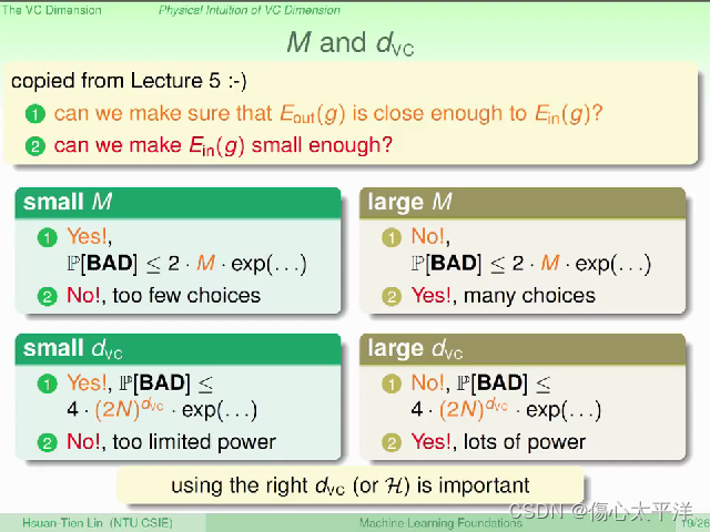
M 与 VC dimension
- 回顾 week 5 时,我们主要想知道的两个问题:
何时会接近
?
- 我们有办法使
- M 与 VC dimension 的取舍
- M,
-
-
但是 h 的选择可能不够多
-
- M,
- h 的选择足够多
-
但
- M,
Video4: Interpreting VC Dimension
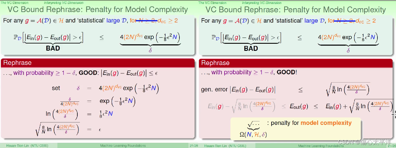
VC Bound Rephrase: Penalty for Model Complexity
- 回顾 VC bound,并试着寻找其他意义
- 把坏事发生几率的上限定为 δ,推导出 ε (其意义为误差容忍值)
- 最后得到
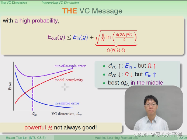
The VC Message
- 随着 VC Dimension 增加,
- 强大的 Hypothesis 并不全然是好事
- 必须找到最佳的 VC Dimension,来得到最低的
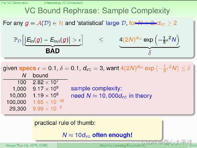
VC Bound Rephrase: Sample Complexity
- 透过霍夫丁不等式,在给定 N, ε,
- 理论上,最好是 N ~ 10000
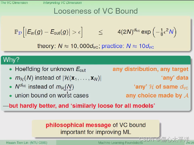
Looseness of VC Bound
- 前面发现理论上与实务上有不小差距,其来源主要来自于:
- 理论没有限制数据的分布、目标函数的形式
- 理论使用的是成长函数,而不是实际的 dichotomies 数量
- 理论使用 VC dimension,因此高估了成长函数上限
- 理论使用 union bound 来计算最坏情况,但实际上最坏情况没那么容易出现


 被折叠的 条评论
为什么被折叠?
被折叠的 条评论
为什么被折叠?
 到【灌水乐园】发言


