


 Loop细分是一种基于三角网格的细分方法,用于使网格模型更光滑。它首先增加顶点,然后通过特定公式调整顶点位置,如内部V-顶点、边界V-顶点和边界E-顶点的位置。在Matlab中可以实现这一过程,相关代码可在链接中找到。
网格细分 —— Loop细分
1. 定义
网格细分是通过按一定规则给网格增加顶点和面片的数量,让网格模型变得更加光滑。Loop细分方法是最早一种基于三角网格的细分方法。一次细分的过程分为两步骤,第一步是增加顶点;第二步是对顶点位置进行调整,使得网格更加光滑。
2. 增加顶点
Loop细分在每条边上都增加一个顶点,并且同一个三角形内的顶点用新增顶点连接起来,以构成新的三角形。
3. 顶点位置的调整
3.1 网格内部V-顶点位置:
对于已经存在的顶点
p
p
p,假定它的度为
n
n
n,它的邻接顶点为
{
p
1
,
p
2
,
…
,
p
n
}
\{p_1,p_2,\dots,p_n\}
{p1,p2,…,pn},则下面的公式更新顶点坐标:
p
′
=
(
1
−
n
β
)
p
+
β
(
p
1
+
p
2
+
⋯
+
p
n
)
p' = (1-n\beta)p+\beta(p_1+p_2+\dots+p_n)
p′=(1−nβ)p+β(p1+p2+⋯+pn)
其中,
β
=
1
n
(
5
8
−
(
3
8
+
1
4
cos
2
π
n
)
2
)
\beta = \frac{1}{n}\left(\frac{5}{8}-(\frac{3}{8}+\frac{1}{4}\cos \frac{2 \pi}{n})^2 \right)
β=n1(85−(83+41cosn2π)2)。
3.2 网络边界V-顶点位置:
对于已经存在的顶点 p p p,假定它的两个相邻点为 p 0 p_0 p0和 p 1 p_1 p1,则该顶点更新后的位置为 p = 6 8 p 0 + 1 8 ( p 1 + p 2 ) p = \frac{6}{8}p_0 + \frac{1}{8}(p_1 + p_2) p=86p0+81(p1+p2)
3.3 网格边界E-顶点位置:
对于新插入的顶点
q
q
q,假设其位于边
p
0
p
1
p_0p_1
p0p1上,
p
2
p_2
p2和
p
3
p_3
p3为边
p
0
p
1
p_0p_1
p0p1对着的第一顶点和第二顶点。则新增的顶点位置为
q
=
3
p
0
+
3
p
1
+
p
2
+
p
3
8
q = \frac{3p_0+3p_1+p_2+p_3}{8}
q=83p0+3p1+p2+p3
3.4 网格边界E-顶点位置:
设边界的两个顶点为
p
0
p_0
p0和
p
1
p_1
p1,则新增加的顶点
q
q
q位置为
q
=
1
2
(
p
0
+
p
1
)
q = \frac{1}{2}(p_0 +p_1)
q=21(p0+p1)
4. Matlab实现
以下代码来自 https://ww2.mathworks.cn/matlabcentral/fileexchange/24942-loop-subdivision
在理解的过程中我添加了些注释,如果有不对的地方希望多多指教。
- loopSubdivision.m
function [newVertices, newFaces] = loopSubdivision(vertices,faces)
    % vertices: 3 * n  顶点:3代表点的坐标(x,y,z)
    % faces: 3 * n     面:3代表三角网格模型中每个三角面顶点,顶点编号为逆时针顺序
    global edgeVertice;
    global newIndexOfVertices;
    newFaces = [];
    newVertices = [];

    nVertices = size(vertices,2); % 顶点个数
    nFaces = size(faces,2);       % 面的个数
    edgeVertice = zeros(nVertices,nVertices,3);  % 边点矩阵
    newIndexOfVertices = nVertices;              % 初始新图形顶点个数

    % ------------------------------------------------------------------------ %
	% 创建一个新的边点矩阵即edgeVertice以及新的三角面newFaces.
    % 时间复杂度 = O(3*nFaces)
    %
    % * edgeVertice(x,y,1): index of the new vertice between (x,y)
    % * edgeVertice(x,y,2): index of the first opposite vertex between (x,y)
    % * edgeVertice(x,y,3): index of the second opposite vertex between (x,y)
    %
    % 一个边最多被两个三角形公用,如果被一个三角形用,那其就是边界,如果被两个三角形共用,就是内部边
    % 原始顶点: va, vb, vc, vd.
    % 新的顶点: vp, vq, vr.
    %
    %      vb                   vb
    %     / \                  /  \
    %    /   \                vp--vq
    %   /     \              / \  / \
    % va ----- vc   ->     va-- vr --vc
    %   \     /              \      /
    %    \   /                \    /
    %     \ /                  \  /
    %      vd                   vd

    for i=1:nFaces
        % deal表示分别给vaIndex,vbIndex,vcIndex赋值
        [vaIndex, vbIndex, vcIndex] = deal(faces(1,i), faces(2,i), faces(3,i));
        vpIndex = addEdgeVertice(vaIndex, vbIndex, vcIndex);
		vqIndex = addEdgeVertice(vbIndex, vcIndex, vaIndex);
		vrIndex = addEdgeVertice(vaIndex, vcIndex, vbIndex);

        fourFaces = [vaIndex,vpIndex,vrIndex; vpIndex,vbIndex,vqIndex; vrIndex,vqIndex,vcIndex; vrIndex,vpIndex,vqIndex]';
		newFaces  = [newFaces, fourFaces]; %加入新的三角面
    end;
    % ------------------------------------------------------------------------ %
	% 更新插入顶点
	for v1=1:nVertices-1
		for v2=v1:nVertices
			vNIndex = edgeVertice(v1,v2,1);
            if (vNIndex~=0)
    			vNOpposite1Index = edgeVertice(v1,v2,2);
        		vNOpposite2Index = edgeVertice(v1,v2,3);
				if (vNOpposite2Index==0) % 边界边
 					newVertices(:,vNIndex) = 1/2*(vertices(:,v1)+vertices(:,v2));
                else  % 内部边
 					newVertices(:,vNIndex) = 3/8*(vertices(:,v1)+vertices(:,v2)) + 1/8*(vertices(:,vNOpposite1Index)+vertices(:,vNOpposite2Index));
                end;
            end;
        end;
    end;
	% ------------------------------------------------------------------------ %
    % adjacent vertices (using edgeVertice)
	adjVertice{nVertices} = []; % 定义长度为n的细胞数组,存储每个点的邻接点
	for v=1:nVertices
		for vTmp=1:nVertices
			if (v<vTmp && edgeVertice(v,vTmp,1)~=0) || (v>vTmp && edgeVertice(vTmp,v,1)~=0)
				adjVertice{v}(end+1) = vTmp;
            end;
        end;
    end;
	% ------------------------------------------------------------------------ %
    % new positions of the original vertices
	for v=1:nVertices
		k = length(adjVertice{v});
		adjBoundaryVertices = []; % 存储边界顶点
		for i=1:k
			vi = adjVertice{v}(i);
			if (vi>v) && (edgeVertice(v,vi,3)==0) || (vi<v) && (edgeVertice(vi,v,3)==0)
				adjBoundaryVertices(end+1) = vi;
			end;
		end;
		if (length(adjBoundaryVertices)==2) % 边界边
			newVertices(:,v) = 6/8*vertices(:,v) + 1/8*sum(vertices(:,adjBoundaryVertices),2);
		else
			beta = 1/k*( 5/8 - (3/8 + 1/4*cos(2*pi/k))^2 );
			newVertices(:,v) = (1-k*beta)*vertices(:,v) + beta*sum(vertices(:,(adjVertice{v})),2);
		end;
    end;
end
- addEdgeVertice.m
function vNIndex = addEdgeVertice(v1Index, v2Index, v3Index)
	global edgeVertice;
	global newIndexOfVertices;
	if (v1Index>v2Index) % setting: v1 <= v2
		vTmp = v1Index;
		v1Index = v2Index;
		v2Index = vTmp;
	end;

	if (edgeVertice(v1Index, v2Index, 1)==0)  % new vertex
		newIndexOfVertices = newIndexOfVertices+1;
		edgeVertice(v1Index, v2Index, 1) = newIndexOfVertices; % 新加入顶点的编号
		edgeVertice(v1Index, v2Index, 2) = v3Index; % 边(v1Index,v2Index)对着的第一个顶点v3Index
	else
		edgeVertice(v1Index, v2Index, 3) = v3Index; % 表示边(v1Index,v2Index)已经被使用过,v3Index是其对着的第二个顶点
	end;
	vNIndex = edgeVertice(v1Index, v2Index, 1);% 返回新加入顶点编号
    return;
end
- test.m
% Test: Mesh subdivision using the Loop scheme.
%
% Author: Jesus Mena
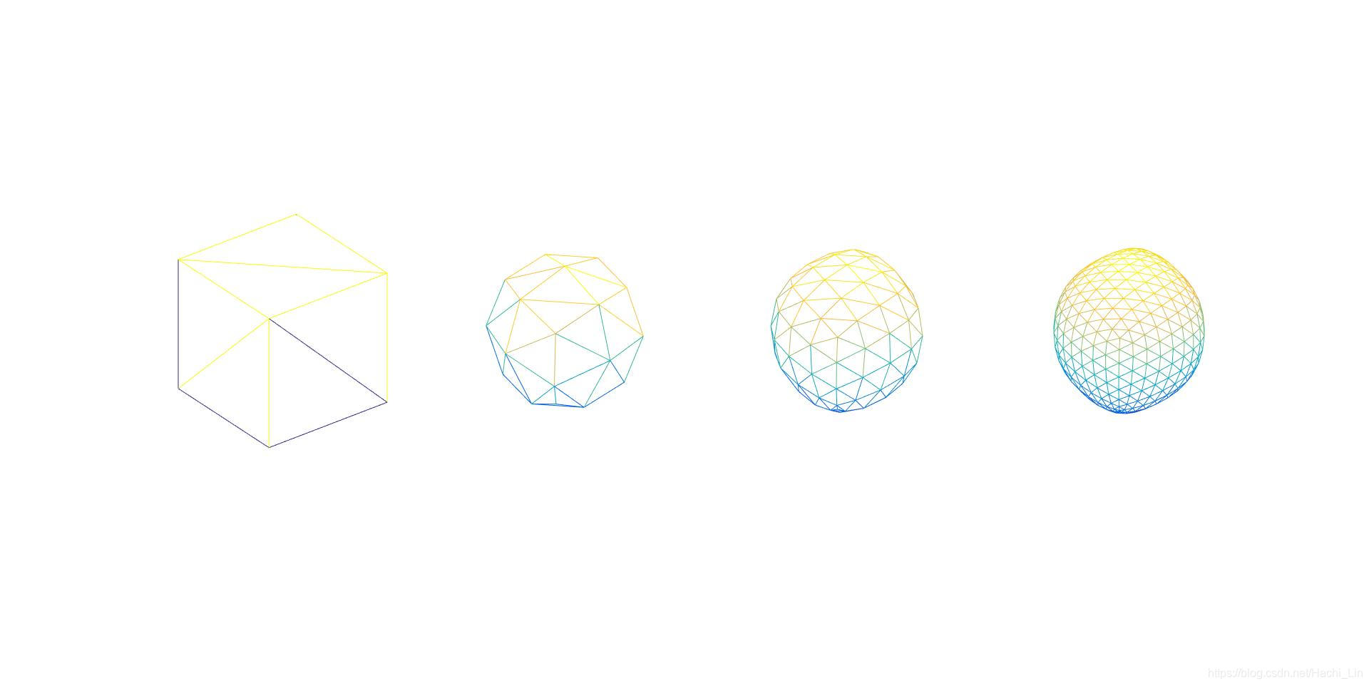
% Example: Box
vertices = [10 10 10; -10 10 10; 10 -10 10; -10 -10 10; 10 10 -10; -10 10 -10; 10 -10 -10; -10 -10 -10]';
faces = [1 2 3; 4 3 2; 1 3 5; 7 5 3; 1 5 2; 6 2 5; 8 6 7; 5 7 6; 8 7 4; 3 4 7; 8 4 6; 2 6 4]';
figure(1);
subplot(1,4,1);
plotMesh(vertices, faces);
for i=2:4
subplot(1,4,i);
[vertices, faces] = loopSubdivision(vertices, faces);
plotMesh(vertices, faces);
end
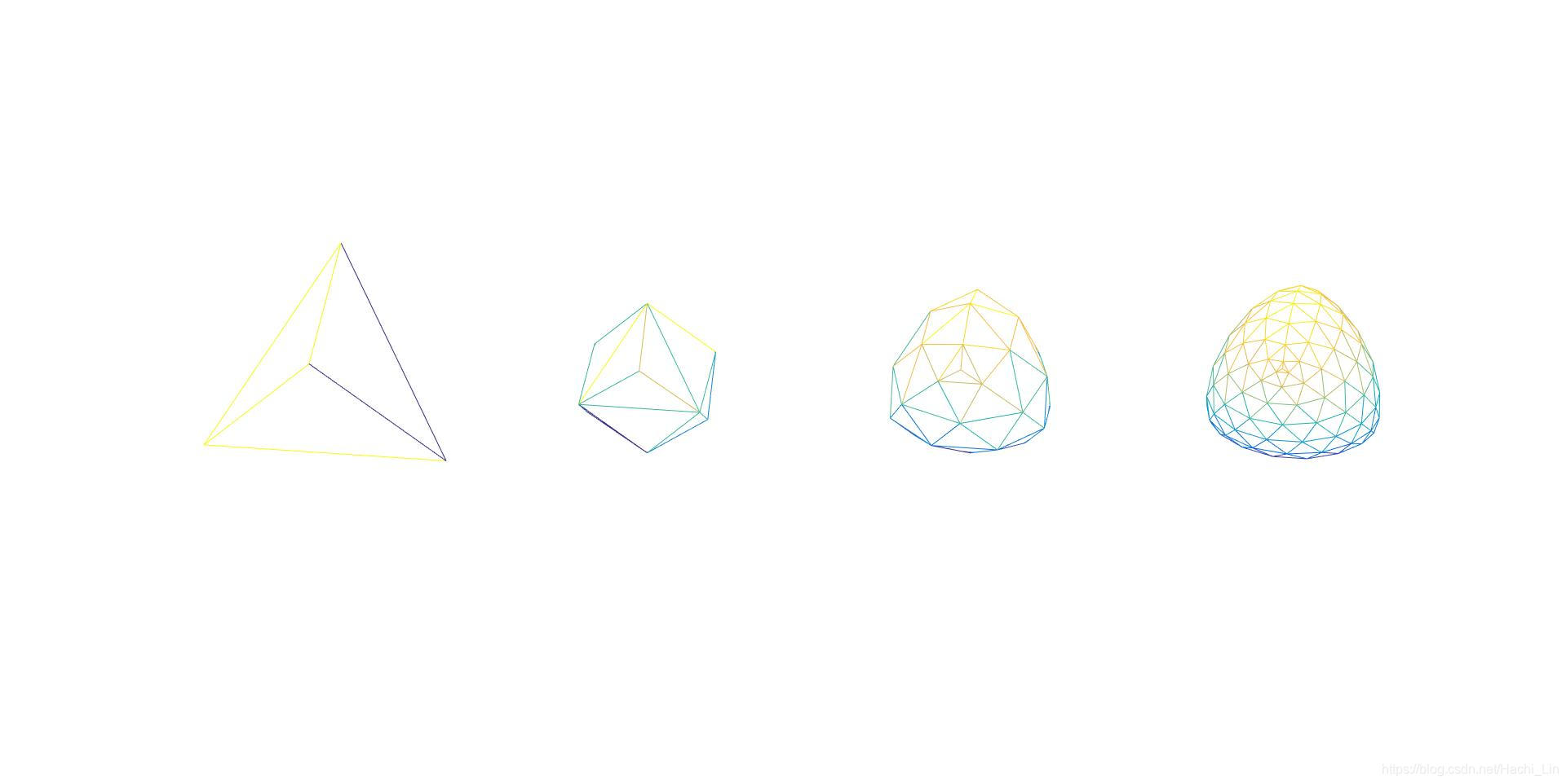
% Example: Tetrahedron
vertices = [10 10 10; -100 10 -10; -100 -10 10; 10 -10 -10]';
faces = [1 2 3; 1 3 4; 1 4 2; 4 3 2]';
figure(2);
subplot(1,4,1);
plotMesh(vertices, faces);
for i=2:4
subplot(1,4,i);
[vertices, faces] = loopSubdivision(vertices, faces);
plotMesh(vertices, faces);
end
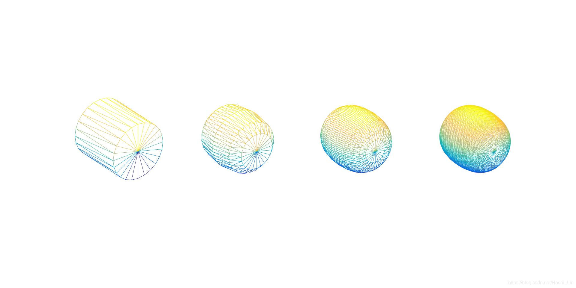
% Example: Cylinder
vertices = [0 -5 0; 0 5 0; 10 -5 0; 9.65 -5 2.58; 8.66 -5 5; 7.07 -5 7.07; 5 -5 8.66; 2.58 -5 9.65; 0 -5 10; -2.58 -5 9.65; -5 -5 8.66; -7.07 -5 7.07; -8.66 -5 5; -9.65 -5 2.58; -10 -5 0; -9.65 -5 -2.58; -8.66 -5 -5; -7.07 -5 -7.07; -5 -5 -8.66; -2.58 -5 -9.65; -0 -5 -10; 2.58 -5 -9.65; 5 -5 -8.66; 7.07 -5 -7.07; 8.66 -5 -5; 9.65 -5 -2.58; 10 5 0 ; 9.65 5 2.58; 8.66 5 5; 7.07 5 7.07; 5 5 8.66; 2.58 5 9.65; 0 5 10; -2.58 5 9.65; -5 5 8.66; -7.07 5 7.07; -8.66 5 5; -9.65 5 2.58; -10 5 0; -9.65 5 -2.58; -8.66 5 -5; -7.07 5 -7.07; -5 5 -8.66; -2.58 5 -9.65; -0 5 -10; 2.58 5 -9.65; 5 5 -8.66; 7.07 5 -7.07; 8.66 5 -5; 9.65 5 -2.58]';
faces = [1 3 4; 1 4 5; 1 5 6; 1 6 7; 1 7 8; 1 8 9; 1 9 10; 1 10 11; 1 11 12; 1 12 13; 1 13 14; 1 14 15; 1 15 16; 1 16 17; 1 17 18; 1 18 19; 1 19 20; 1 20 21; 1 21 22; 1 22 23; 1 23 24; 1 24 25; 1 25 26; 1 26 3; 2 28 27; 2 29 28; 2 30 29; 2 31 30; 2 32 31; 2 33 32; 2 34 33; 2 35 34; 2 36 35; 2 37 36; 2 38 37; 2 39 38; 2 40 39; 2 41 40; 2 42 41; 2 43 42; 2 44 43; 2 45 44; 2 46 45; 2 47 46; 2 48 47; 2 49 48; 2 50 49; 2 27 50; 3 27 28; 3 28 4; 4 28 29; 4 29 5; 5 29 30; 5 30 6; 6 30 31; 6 31 7; 7 31 32; 7 32 8; 8 32 33; 8 33 9; 9 33 34; 9 34 10; 10 34 35; 10 35 11; 11 35 36; 11 36 12; 12 36 37; 12 37 13; 13 37 38; 13 38 14; 14 38 39; 14 39 15; 15 39 40; 15 40 16; 16 40 41; 16 41 17; 17 41 42; 17 42 18; 18 42 43; 18 43 19; 19 43 44; 19 44 20; 20 44 45; 20 45 21; 21 45 46; 21 46 22; 22 46 47; 22 47 23; 23 47 48; 23 48 24; 24 48 49; 24 49 25; 25 49 50; 25 50 26; 26 50 27; 26 27 3]';
figure(3);
subplot(1,4,1);
plotMesh(vertices, faces);
for i=2:4
subplot(1,4,i);
[vertices, faces] = loopSubdivision(vertices, faces);
plotMesh(vertices, faces);
end
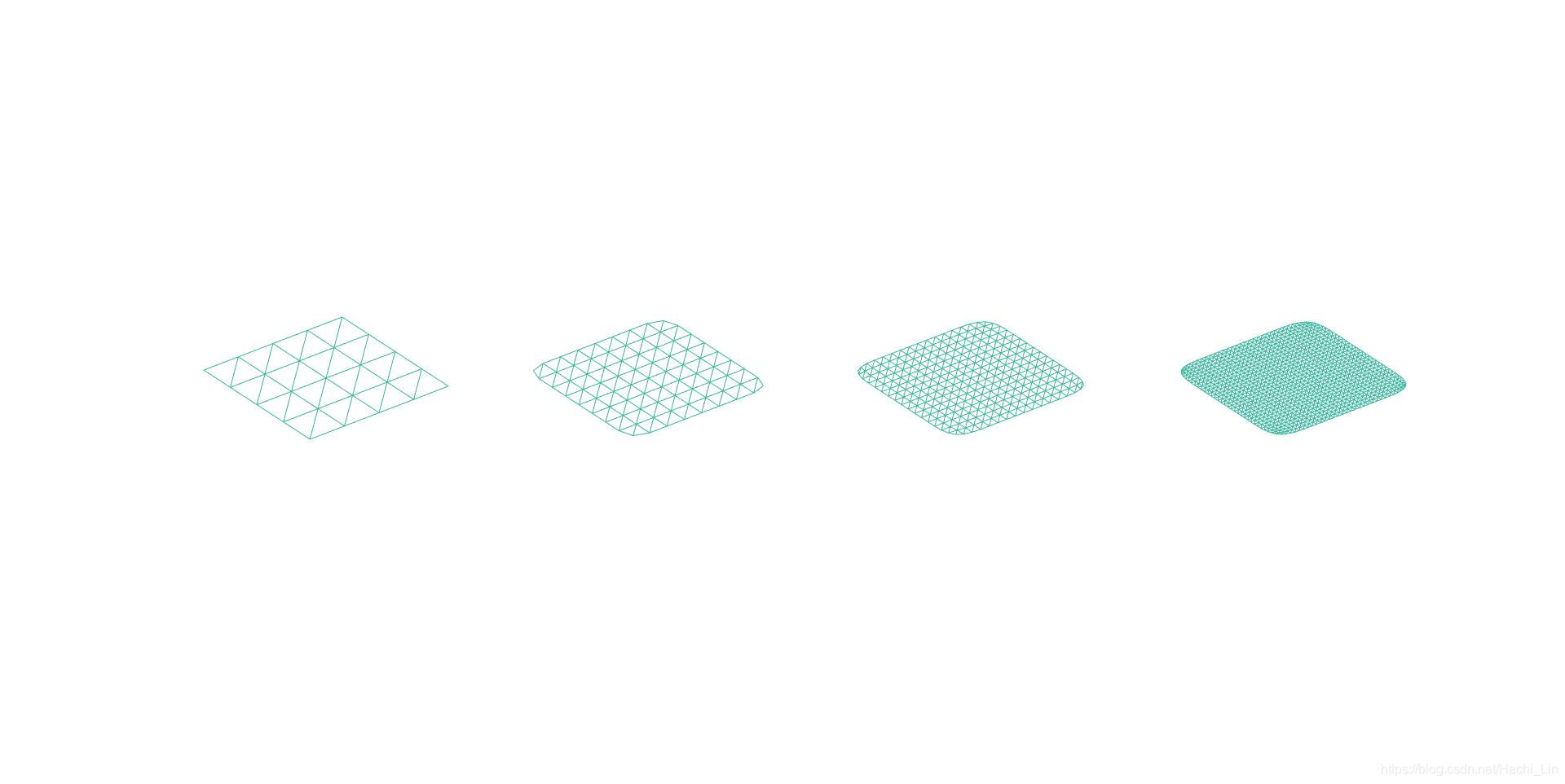
% Example: Grid
vertices = [-4 -4 0; -2 -4 0; 0 -4 0; 2 -4 0; 4 -4 0; -4 -2 0; -2 -2 0; 0 -2 0; 2 -2 0; 4 -2 0; -4 0 0; -2 0 0; 0 0 0; 2 0 0; 4 0 0; -4 2 0; -2 2 0; 0 2 0; 2 2 0; 4 2 0; -4 4 0; -2 4 0; 0 4 0; 2 4 0; 4 4 0]';
faces = [7 2 1; 1 6 7; 8 3 2; 2 7 8; 9 4 3; 3 8 9; 10 5 4; 4 9 10; 12 7 6; 6 11 12; 13 8 7; 7 12 13; 14 9 8; 8 13 14; 15 10 9; 9 14 15; 17 12 11; 11 16 17; 18 13 12; 12 17 18; 19 14 13; 13 18 19; 20 15 14; 14 19 20; 22 17 16; 16 21 22; 23 18 17; 17 22 23; 24 19 18; 18 23 24; 25 20 19; 19 24 25]';
figure(4);
subplot(1,4,1);
plotMesh(vertices, faces);
for i=2:4
subplot(1,4,i);
[vertices, faces] = loopSubdivision(vertices, faces);
plotMesh(vertices, faces);
end
- plotMesh.m
function plotMesh(vertices, faces)
    hold on;
    trimesh(faces', vertices(1,:), vertices(2,:), vertices(3,:));
    colormap gray(1);
    axis tight;   % 将坐标范围设定为被绘制的数据范围
    axis square;  % 将坐标轴设置为正方形
    axis off;     % 关闭所有的坐标轴标签、刻度、背景
    view(3);      % 设置默认的三维视角
end
- 结果
- figure1
- figure2
- figure3
- figure4
5. 有用的链接
https://blog.youkuaiyun.com/lafengxiaoyu/article/details/51581801
https://www.cnblogs.com/shushen/p/5251070.html


 662
662

 被折叠的 条评论
为什么被折叠?
被折叠的 条评论
为什么被折叠?
 到【灌水乐园】发言


