


💥💥💞💞欢迎来到本博客❤️❤️💥💥
🏆博主优势:🌞🌞🌞博客内容尽量做到思维缜密,逻辑清晰,为了方便读者。
⛳️座右铭:行百里者,半于九十。
📋📋📋本文目录如下:🎁🎁🎁
目录
💥1 概述
非线性模型预测控制(Model Predictive Control, MPC)是一种常用的控制方法,可以应用于多种系统,包括非线性系统。MPC基于离散化的模型和未来时间段的优化问题,通过迭代地求解优化问题来生成控制策略。
一、研究背景与意义
非线性模型预测控制(Nonlinear Model Predictive Control, NMPC)是一种基于非线性模型的闭环优化控制策略,适用于处理具有强非线性、多变量、时变及约束条件的复杂系统控制问题。随着工业过程复杂化、大型化及智能化的发展,传统线性MPC方法在处理非线性系统时面临精度不足、鲁棒性差等挑战。NMPC通过建立非线性动态模型,在每个采样周期内求解有限时域优化问题,生成最优控制序列,并仅应用当前时刻的控制输入,实现滚动优化与反馈校正,从而显著提升非线性系统的控制性能。
二、NMPC基本原理与数学框架
- 系统模型
NMPC依赖非线性动态模型描述系统行为,常见模型形式包括:- 第一原理模型:基于物理定律(如守恒方程)构建,适用于机理明确的系统(如化学反应器)。
- 黑箱模型:通过数据驱动方法(如神经网络、模糊系统)构建,适用于机理复杂的系统。
- 混合模型:结合第一原理与数据驱动方法,平衡精度与计算复杂度。
- 最优控制律
在每个采样时刻,NMPC求解以下优化问题:-
目标函数:最小化系统状态跟踪误差、控制输入幅值等性能指标,例如:
-
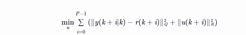
其中,y为系统输出,r为参考轨迹,Q和R为权重矩阵,P为预测时域。 |
- 约束条件:包括状态约束、输入约束及输出约束,确保系统安全稳定运行。
- 滚动优化:仅应用最优序列的第一个控制输入,并在下一时刻重新优化,通过反馈校正增强鲁棒性。
- 稳定性与鲁棒性
- 通过引入终端约束(Terminal Constraint)或终端代价函数(Terminal Cost)保证闭环稳定性,但设计难度随系统非线性程度增加。
- 鲁棒NMPC方法(如Tube-based MPC)通过处理模型不确定性,提升系统对外部干扰的适应能力。
三、NMPC问题求解方法
- 数值优化算法
- 序列二次规划(SQP):通过迭代求解二次子问题逼近最优解,适合中等规模问题,但需处理Hessian矩阵计算,对初值敏感。
- 内点法(IPM):通过引入障碍函数处理约束,适合大规模问题,但对初值选择要求较高。
- C/GMRES方法:结合连续化与广义最小残差法,实时性强,适用于快速动态系统(如无人机)。
- 启发式算法
- 遗传算法(GA)、混沌灰狼优化(CGWO)等全局搜索能力强,但计算效率较低,适用于离线优化或简单系统。
- 加速求解策略
- 热启动(Warm Start):利用上一时刻的解作为初值,减少迭代次数。
- 并行计算:利用GPU或多核CPU加速矩阵运算。
- 模型简化:通过降阶模型(如POD)或线性化降低复杂度,但可能牺牲精度。
- 控制器设计简化
- 次优设计:牺牲全局最优性以换取实时性,通过可行解保证稳定性。
- 参数化控制律:将控制输入参数化为有限维函数(如多项式基函数),降低决策变量维度。
- 混合控制策略:结合NMPC与线性MPC或反馈控制器,平衡性能与计算负载。
四、NMPC典型应用案例
- 机器人控制
- 自动泊车:通过预测车辆运动学模型,优化转向角与速度,实现高精度路径跟踪。
- 机械臂轨迹跟踪:矿区洒水车机械臂采用NMPC后,位移误差降低89.85%,解算时间<8.7ms。
- 无人系统
- 无人机轨迹跟踪:NMPC在复杂轨迹(如双移线)中表现优于PID,但需更高计算资源。
- 四旋翼控制:结合动力学模型与障碍函数,实现避障与稳定飞行。
- 工业过程控制
- 化工反应器:NMPC优化温度与浓度约束,提高反应效率。
- 能源管理:在燃料电池混合动力车中,NMPC通过RNN模型实现最大效率点跟踪,燃料经济性优于线性MPC。
- 交通与车辆
- 无人驾驶轨迹跟踪:NMPC处理非线性轮胎力模型,适应弯道与紧急制动场景。
- 集成式决策控制:动态调整需求指标优先级,实现高实时性(单步求解<50ms)的自动驾驶。
五、当前研究热点与挑战
- 计算效率提升
- 开发稀疏SQP、分布式NMPC等算法,降低时间复杂度。
- 利用FPGA或边缘计算设备实现嵌入式部署。
- 鲁棒性与适应性增强
- 采用Tube-based或Min-Max方法处理模型不确定性。
- 结合贝叶斯估计或粒子滤波,实时更新模型参数。
- 复杂系统扩展
- 多智能体协同:研究分布式NMPC框架,解决通信与耦合约束。
- 高维状态空间:利用深度学习压缩状态维度,如自编码器。
- 实时性与稳定性平衡
- 次优性分析:量化次优解对闭环性能的影响。
- 安全验证:引入形式化方法(如Barrier Function)保证硬约束满足。
六、未来研究方向
- 算法-硬件协同设计
- 结合定制化芯片与高效算法,满足毫秒级实时需求。
- 混合架构创新
- 融合NMPC与强化学习、自适应控制,提升动态环境适应性。
- 标准化工具链开发
- 提供开源框架(如ACADO、CasADi)的工业级支持,降低工程落地门槛。
- 数据驱动与模型融合
- 利用高斯过程回归、神经网络等数据驱动方法,提升模型精度与泛化能力。
七、结论
NMPC凭借其处理非线性和约束的能力,在工业过程控制、机器人、航空航天等领域取得显著应用成果。然而,其在计算复杂度、模型精度、鲁棒性及实时性方面仍面临挑战。未来研究将聚焦于算法优化、硬件加速、混合控制策略及标准化工具开发,推动NMPC在智能制造、新能源、自动驾驶等领域的广泛应用。
📚2 运行结果


可视化:
% Plot the results

% Plant: Controlled by PI controller
% Strip off last computed value of h
hhp=hp(timeref);

figure(2)
clf
subplot(211)
plot(time,hhp,'k-',time,ref,'b--')
grid
ylabel('Liquid height, h')
title('Liquid level h and reference input r (plant)')

subplot(212)
plot(time,up,'k-')
grid
title('Tank input, u')
xlabel('Time, k')
axis([min(time) max(time) -50 50])

% Model: Controlled by PI controller
% Strip off last computed value of hmm
hhm=hmm(timeref);

figure(3)
clf
subplot(211)
plot(time,hhm,'k-',time,ref,'k--')
grid
ylabel('Liquid height, h_m')
title('Liquid level h_m and reference input r (model)')

subplot(212)
plot(time,umm,'k-')
grid
title('Tank input, u_m')
xlabel('Time, k')
axis([min(time) max(time) -50 50])

% Difference between plant and model: Controlled by PI controller
% Strip off last computed value of hmm

figure(4)
clf
subplot(211)
plot(time,hhp-hhm,'k-')
grid
title('Liquid height error')

subplot(212)
plot(time,up-umm,'k-')
grid
title('Tank input error')
xlabel('Time, k')


%-----------------------------------------------------------
% Planning system results
% Strip off last computed value of h
hh=h(timeref);

figure(5)
clf
subplot(211)
plot(time,hh,'k-',time,ref,'k--')
grid
ylabel('Liquid height, h')
title('Liquid level h and reference input r')

subplot(212)
plot(time,u,'k-')
grid
title('Tank input, u')
xlabel('Time, k')
axis([min(time) max(time) -50 50])

figure(6)
clf
plot(time,rowindex,'k-',time,colindex,'k--')
axis([min(time) max(time) 0 max(length(Kpvec),length(Kivec))])
grid
title('Indices of plan (row=solid, column=dashed)')
ylabel('Row and column indices')
xlabel('Time, k')

% Next, study the effect of the projection length N
figure(7)
clf
plot(NN,trackerrorenergy,'b-',NN,trackerrorenergy,'ro')
title('Tracking energy vs. projection length N')
xlabel('Projection length N')

figure(8)
clf
plot(NN,inputenergy,'b-',NN,inputenergy,'ro')
title('Control energy vs. projection length N')
xlabel('Projection length N')

%%%%%%%%%%%%%%%%%%%%%%%%%%%%%%%%%%%%%%%%%%%%%%%%%%%%%%%%%%%%%%%%%%%%%%%%%
% End of program
%%%%%%%%%%%%%%%%%%%%%%%%%%%%%%%%%%%%%%%%%%%%%%%%%%%%%%%%%%%%%%%%%%%%%%%%%
% Plot the results
% Plant: Controlled by PI controller
% Strip off last computed value of h
hhp=hp(timeref);
figure(2)
clf
subplot(211)
plot(time,hhp,'k-',time,ref,'b--')
grid
ylabel('Liquid height, h')
title('Liquid level h and reference input r (plant)')
subplot(212)
plot(time,up,'k-')
grid
title('Tank input, u')
xlabel('Time, k')
axis([min(time) max(time) -50 50])
% Model: Controlled by PI controller
% Strip off last computed value of hmm
hhm=hmm(timeref);
figure(3)
clf
subplot(211)
plot(time,hhm,'k-',time,ref,'k--')
grid
ylabel('Liquid height, h_m')
title('Liquid level h_m and reference input r (model)')
subplot(212)
plot(time,umm,'k-')
grid
title('Tank input, u_m')
xlabel('Time, k')
axis([min(time) max(time) -50 50])
% Difference between plant and model: Controlled by PI controller
% Strip off last computed value of hmm
figure(4)
clf
subplot(211)
plot(time,hhp-hhm,'k-')
grid
title('Liquid height error')
subplot(212)
plot(time,up-umm,'k-')
grid
title('Tank input error')
xlabel('Time, k')
%-----------------------------------------------------------
% Planning system results
% Strip off last computed value of h
hh=h(timeref);
figure(5)
clf
subplot(211)
plot(time,hh,'k-',time,ref,'k--')
grid
ylabel('Liquid height, h')
title('Liquid level h and reference input r')
subplot(212)
plot(time,u,'k-')
grid
title('Tank input, u')
xlabel('Time, k')
axis([min(time) max(time) -50 50])
figure(6)
clf
plot(time,rowindex,'k-',time,colindex,'k--')
axis([min(time) max(time) 0 max(length(Kpvec),length(Kivec))])
grid
title('Indices of plan (row=solid, column=dashed)')
ylabel('Row and column indices')
xlabel('Time, k')
% Next, study the effect of the projection length N
figure(7)
clf
plot(NN,trackerrorenergy,'b-',NN,trackerrorenergy,'ro')
title('Tracking energy vs. projection length N')
xlabel('Projection length N')
figure(8)
clf
plot(NN,inputenergy,'b-',NN,inputenergy,'ro')
title('Control energy vs. projection length N')
xlabel('Projection length N')
%%%%%%%%%%%%%%%%%%%%%%%%%%%%%%%%%%%%%%%%%%%%%%%%%%%%%%%%%%%%%%%%%%%%%%%%%
% End of program
%%%%%%%%%%%%%%%%%%%%%%%%%%%%%%%%%%%%%%%%%%%%%%%%%%%%%%%%%%%%%%%%%%%%%%%%%
🎉3 参考文献
文章中一些内容引自网络,会注明出处或引用为参考文献,难免有未尽之处,如有不妥,请随时联系删除。
[1]修观.非线性模型预测控制方法在滑翔弹道控制中的应用研究[D].南京理工大学,2011.DOI:10.7666/d.y1919740.
[2]陈垣君.基于LPV模型非线性预测控制的精细化建模及精确求解[D].浙江大学,2015.
[3]谢树光.非线性模型预测控制(NMPC)在微型飞行器自适应控制中的应用[J]. 2002.


 571
571

 被折叠的 条评论
为什么被折叠?
被折叠的 条评论
为什么被折叠?
 到【灌水乐园】发言


