【slingshot and tradeSeq】differential analysis between different lineages

tradeSeq是同一团队做的R包，主要功能有：

（1）比较不同conditions的lineages.例如一组mock stimulation, 一组TGF stimulation,检验两个lineages是否分布相同，如果不相同，可以做差异分析

（2）同一个lineage的不同branch，也可以做差异分析

bioconductor workshop讲解，很好

https://www.youtube.com/watch?v=Fbd08bIv4yk

tutorial 作者提到里面一些功能还处于beta版(2020年时, v0.9)，可以从github安装。bioconductor上成熟的功能也不少，应该是已经发布了(v1.8)。

Trajectory inference across conditions: differential expression and differential progression • bioc2020trajectories

Bioconductor - tradeSeq

另外，在本教程中，integration等上游分析用的Seurat，核心slingshot又回归到了SingleCellExperiment-bioconductor体系，之中有两句代码完成了从seurat到sce的转换 

本文章将综合bioconductor-tradeSeq上的三个教程，完成slingshot拟时序分析-tradeSeq差异分析的pipeline。分成两个部分：（1）tradeSeq的workflow（2）拟合模型时的特殊注意事项。

• 概述

示例数据集为展示上皮-间质转化的细胞，一组TGF刺激，另一组mock stimulation。所以是两种conditions下的single lineage分析。

• the tradeSeq workflow

（1）载入数据

需要准备三个数据：表达矩阵（行为基因列为细胞）、细胞类型注释信息（字符串，与列名顺序一致）、上游做完slingshot后的slingshot S4 object.

library(tradeSeq)
library(RColorBrewer)
library(SingleCellExperiment)
library(slingshot)

# For reproducibility
RNGversion("3.5.0")
palette(brewer.pal(8, "Dark2"))
data(countMatrix, package = "tradeSeq")
counts <- as.matrix(countMatrix)
rm(countMatrix)
data(crv, package = "tradeSeq")
data(celltype, package = "tradeSeq")

（2）fit negative binomial generalized additive model (NB-GAM)

首先通过evaluateK功能决定k值（the number of knots）

set.seed(5)
icMat <- evaluateK(counts = counts, sds = crv, k = 3:10, 
                   nGenes = 200, verbose = T)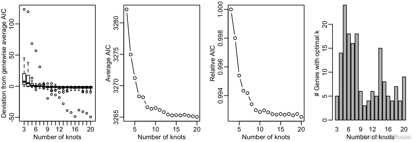

简而言之，在图二中AIC值下降的趋势中止时的K值就是我们要选择的。Here, we pick nknots = 6. 然后用fitGAM功能拟合模型

set.seed(7)

pseudotime <- slingPseudotime(crv, na = FALSE)
cellWeights <- slingCurveWeights(crv)
sce <- fitGAM(counts = counts, pseudotime = pseudotime, cellWeights = cellWeights,
                 nknots = 6, verbose = FALSE)

#检查一下多少基因fit上了
table(rowData(sce)$tradeSeq$converged)

• within lineage comparison

（1）the association of gene expression with pseudotime

This can be interpreted as testing whether the average gene expression is significantly changing along pseudotime.

assoRes <- associationTest(sce)
head(assoRes)

 （2）discovering progenitor marker genes

本质上是progenitor cell（starting cell）和 differentiated cell之间的差异分析

The function startVsEndTest uses a Wald test to assess the null hypothesis that the average expression at the starting point of the smoother (progenitor population) is equal to the average expression at the end point of the smoother (differentiated population). 

默认所有lineages，lineages=TRUE时分别获得。

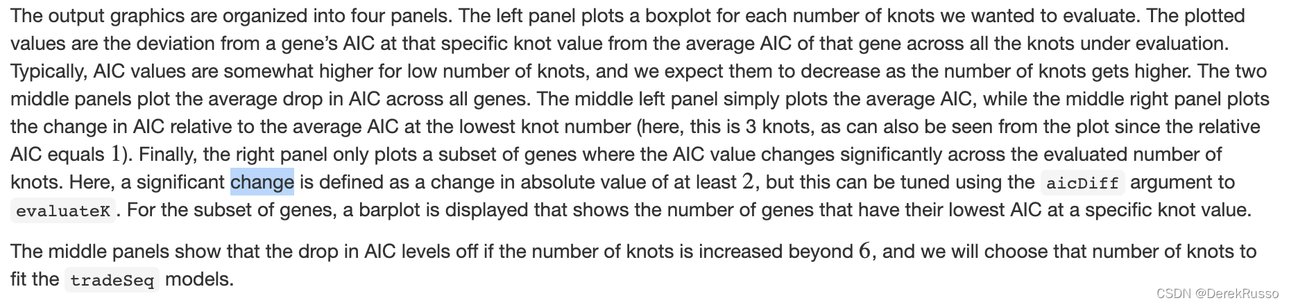
#We can visualize the estimated smoothers for the third most significant gene.

oStart <- order(startRes$waldStat, decreasing = TRUE)
sigGeneStart <- names(sce)[oStart[3]]
plotSmoothers(sce, counts, gene = sigGeneStart)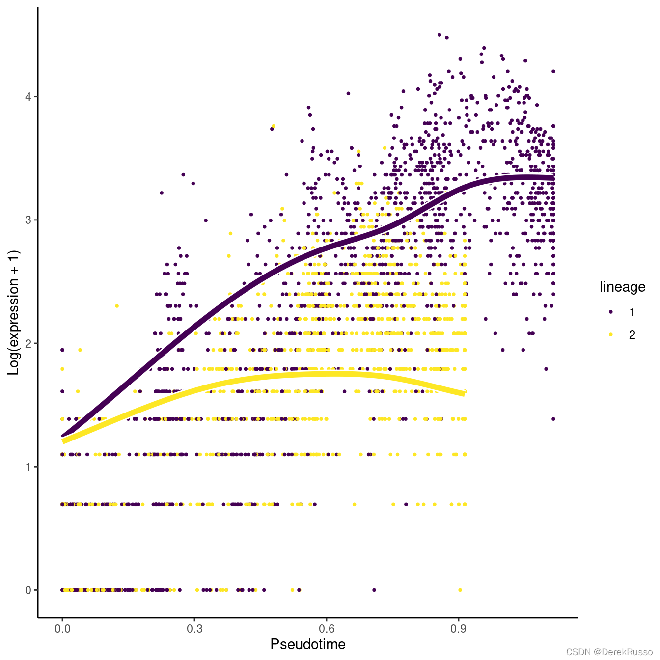

plotGeneCount(crv, counts, gene = sigGeneStart)

 前面功能默认是对起始和终末这两个时间点进行差异分析，还可以自行指定两个时间点。

customRes <- startVsEndTest(sce, pseudotimeValues = c(0.1, 0.8))

• between lineage comparisons

（1）discovering differentiated cell type markers

本质上是对每个lineages的endpoints作差异分析。如果多于两个lineages，加上pairwise=TRUE来做两两对比

endRes <- diffEndTest(sce)

#plot the most significant genes

o <- order(endRes$waldStat, decreasing = TRUE)
sigGene <- names(sce)[o[1]]
plotSmoothers(sce, counts, sigGene)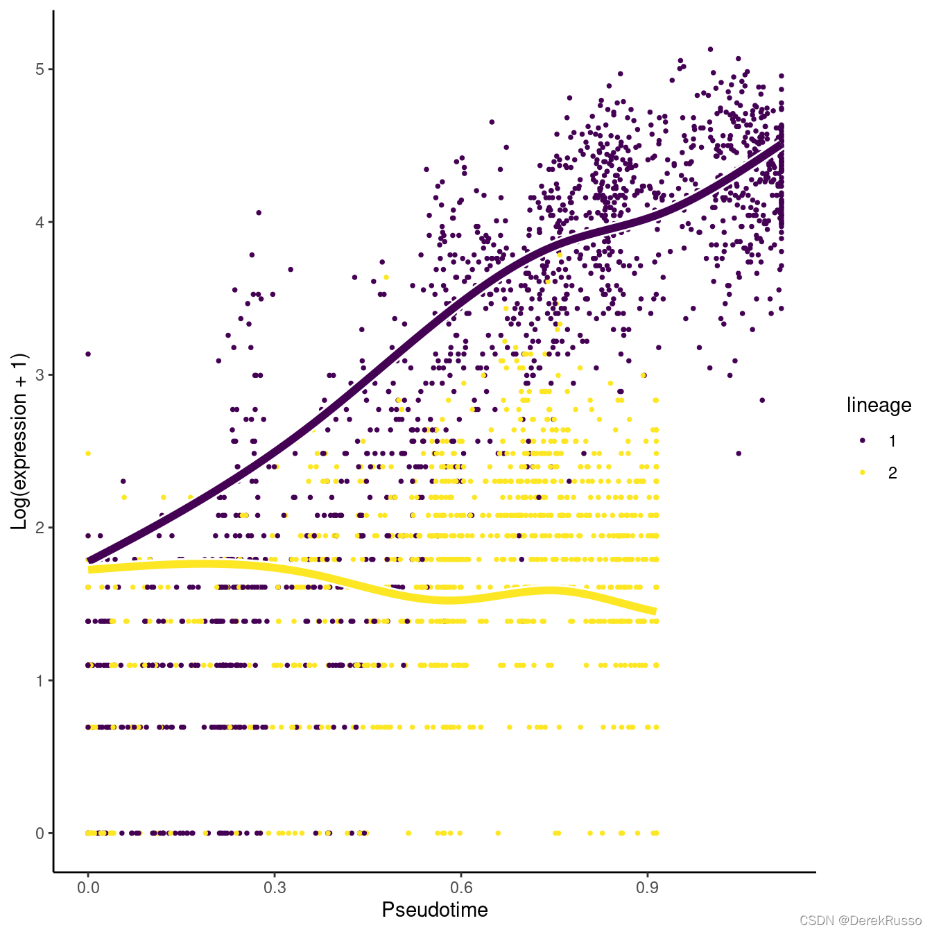

plotGeneCount(crv, counts, gene = sigGene)

（2）discovering genes with different expression patterns

本质上，对某个基因，探究在两个lineages中随着pseudotime的变化，它的表达模式是否不同。

patternRes <- patternTest(sce)
oPat <- order(patternRes$waldStat, decreasing = TRUE)
head(rownames(patternRes)[oPat])

plotSmoothers(sce, counts, gene = rownames(patternRes)[oPat][4])

plotGeneCount(crv, counts, gene = rownames(patternRes)[oPat][4])

有一些基因非常特别，他们在两个lineages中的表达模式（pattern）不同，但在两个终末分化的end points的差异分析中并不差异表达。详情参看文档。

（3）early drivers of differentiation

plotGeneCount(curve = crv, counts = counts,
              clusters = apply(slingClusterLabels(crv), 1, which.max),
              models = sce)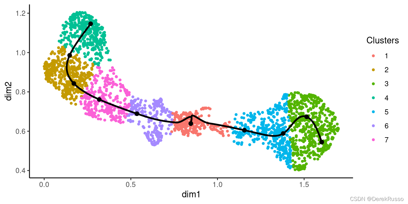

earlyDERes <- earlyDETest(sce, knots = c(1, 2))
oEarly <- order(earlyDERes$waldStat, decreasing = TRUE)
head(rownames(earlyDERes)[oEarly])

plotSmoothers(sce, counts, gene = rownames(earlyDERes)[oEarly][2])

plotGeneCount(crv, counts, gene = rownames(earlyDERes)[oEarly][2])

• clustering of genes according to their expression pattern

另外，tradeSeq还可以做两个condition之间的差异分析

https://kstreet13.github.io/bioc2020trajectories/articles/workshopTrajectories.html