【slingshot】trajectory inference

condiments Paper • condimentsPaper

First example: TGF-beta dataset • bioc2021trajectories

 

slingshot requires a minimum of two inputs: (1)a matrix representing the cells in a reduced-dimensional space. (2)a vector of cluster labels.

主要步骤：

（1）getLineages function to identify global lineage structrue by construsting MST on the clusters

（2）getCurves function to construct smooth curves and infer the psudotime variable

• simulated dataset 1 (single trajectory) and dataset 2 (bifurcating)

#####dataset1
# generate synthetic count data representing a single lineage
means <- rbind(
    # non-DE genes
    matrix(rep(rep(c(0.1,0.5,1,2,3), each = 300),100),
        ncol = 300, byrow = TRUE),
    # early deactivation
    matrix(rep(exp(atan( ((300:1)-200)/50 )),50), ncol = 300, byrow = TRUE),
    # late deactivation
    matrix(rep(exp(atan( ((300:1)-100)/50 )),50), ncol = 300, byrow = TRUE),
    # early activation
    matrix(rep(exp(atan( ((1:300)-100)/50 )),50), ncol = 300, byrow = TRUE),
    # late activation
    matrix(rep(exp(atan( ((1:300)-200)/50 )),50), ncol = 300, byrow = TRUE),
    # transient
    matrix(rep(exp(atan( c((1:100)/33, rep(3,100), (100:1)/33) )),50), 
        ncol = 300, byrow = TRUE)
)
counts <- apply(means,2,function(cell_means){
    total <- rnbinom(1, mu = 7500, size = 4)
    rmultinom(1, total, cell_means)
})
rownames(counts) <- paste0('G',1:750)
colnames(counts) <- paste0('c',1:300)
sce <- SingleCellExperiment(assays = List(counts = counts))


#####dataset2
library(slingshot, quietly = FALSE)
data("slingshotExample")
rd <- slingshotExample$rd
cl <- slingshotExample$cl

dim(rd) # data representing cells in a reduced dimensional space

• upstream analysis

（1）gene filtering

# filter genes down to potential cell-type markers
# at least M (15) reads in at least N (15) cells
geneFilter <- apply(assays(sce)$counts,1,function(x){
    sum(x >= 3) >= 10
})
sce <- sce[geneFilter, ]

（2）normalization

normalization可以选择不同方法，并根据不同方法选择noemalization在pipeline里的顺序，例如MNN是先降维在去除batch effect.作者推荐用scone package,模拟数据用quantile normalization.

FQnorm <- function(counts){
    rk <- apply(counts,2,rank,ties.method='min')
    counts.sort <- apply(counts,2,sort)
    refdist <- apply(counts.sort,1,median)
    norm <- apply(rk,2,function(r){ refdist[r] })
    rownames(norm) <- rownames(counts)
    return(norm)
}
assays(sce)$norm <- FQnorm(assays(sce)$counts)

（3）降维

示例两种方法：PCA, UMAP

pca <- prcomp(t(log1p(assays(sce)$norm)), scale. = FALSE)
rd1 <- pca$x[,1:2]

plot(rd1, col = rgb(0,0,0,.5), pch=16, asp = 1)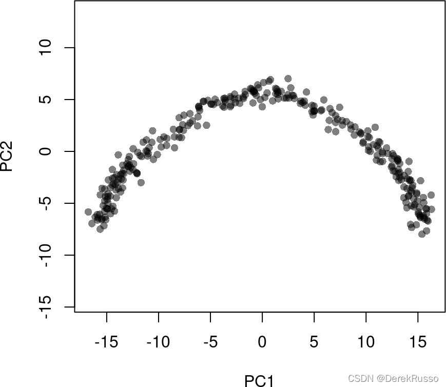

library(uwot)

rd2 <- uwot::umap(t(log1p(assays(sce)$norm)))
colnames(rd2) <- c('UMAP1', 'UMAP2')

plot(rd2, col = rgb(0,0,0,.5), pch=16, asp = 1)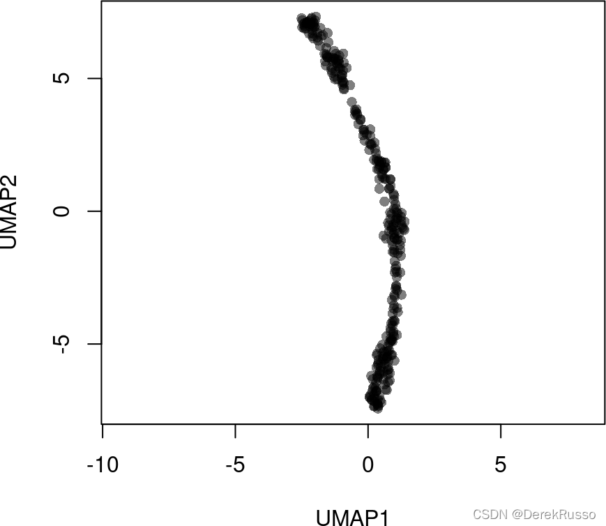

 

##把两种降维结果都加进sce object，但后续分析用pca结果
reducedDims(sce) <- SimpleList(PCA = rd1, UMAP = rd2)

 （3）clustering

两种方法：gaussian mixture modeling (示例) or k-means

library(mclust, quietly = TRUE)

cl1 <- Mclust(rd1)$classification
colData(sce)$GMM <- cl1

library(RColorBrewer)
plot(rd1, col = brewer.pal(9,"Set1")[cl1], pch=16, asp = 1)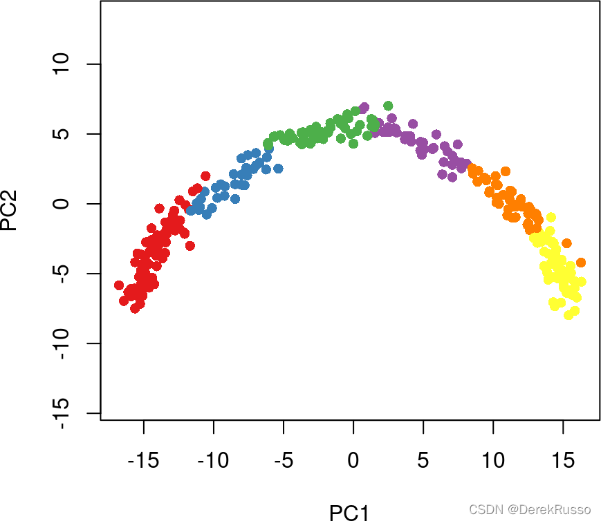

•  using slingshot

本质上是两部，第一步发现global structure,第二步fitting simultaneous principal curves.既可以用wrapper function "slingshot" 一句命令就搞定（作者推荐）；也可以先后用“getLineages”和“getCurves”两句命令。下面单轨迹dataset用wrapper命令，双轨迹dataset用后两个命令分步完成。

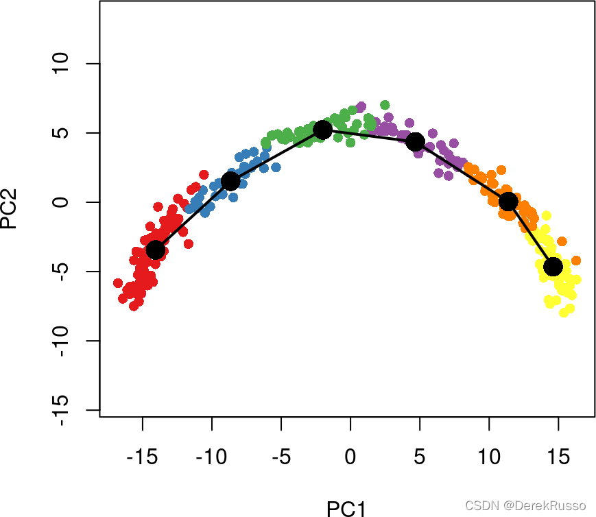
sce <- slingshot(sce, clusterLabels = 'GMM', reducedDim = 'PCA')

visualize the result

summary(sce$slingPseudotime_1)

library(grDevices)
colors <- colorRampPalette(brewer.pal(11,'Spectral')[-6])(100)
plotcol <- colors[cut(sce$slingPseudotime_1, breaks=100)]

plot(reducedDims(sce)$PCA, col = plotcol, pch=16, asp = 1)
lines(SlingshotDataSet(sce), lwd=2, col='black')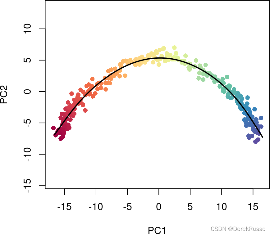

#We can also see how the lineage structure was intially estimated by the cluster-based minimum spanning tree

plot(reducedDims(sce)$PCA, col = brewer.pal(9,'Set1')[sce$GMM], pch=16, asp = 1)
lines(SlingshotDataSet(sce), lwd=2, type = 'lineages', col = 'black')

• downstream analysis (identifying temporally dynamic genes)

library(tradeSeq)

# fit negative binomial GAM
sce <- fitGAM(sce)

# test for dynamic expression
ATres <- associationTest(sce)

We can then pick out the top genes based on p-values and visualize their expression over developmental time with a heatmap. Here we use the top 250 most dynamically expressed genes.

topgenes <- rownames(ATres[order(ATres$pvalue), ])[1:250]
pst.ord <- order(sce$slingPseudotime_1, na.last = NA)
heatdata <- assays(sce)$counts[topgenes, pst.ord]
heatclus <- sce$GMM[pst.ord]

heatmap(log1p(heatdata), Colv = NA,
        ColSideColors = brewer.pal(9,"Set1")[heatclus])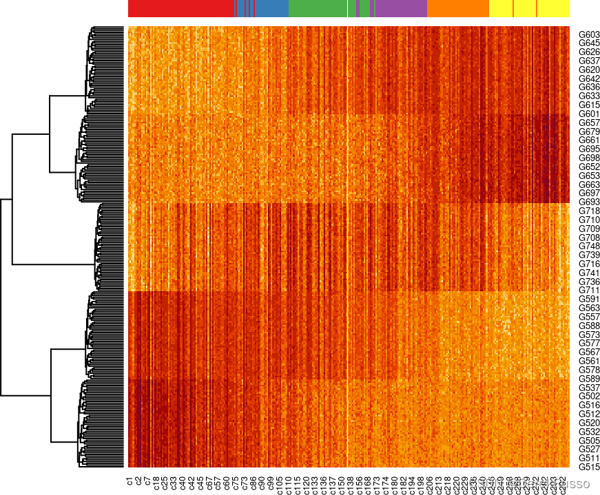

 

• Detailed slingshot functionalities 

为了更好的解释slingshot的其他功能，以下开始用slingshot自带的第二个数据集（bifurcating），并且直接将low dimensional matrix (by k-means)和cluster labels 作为输入，而非先构建sce object.因为后者还需要表达矩阵。

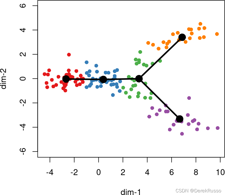
（1）identifying global lineage structure

The getLineages function takes as input an n ×× p matrix and a vector of clustering results of length n.

This analysis can be performed in an entirely unsupervised manner or in a semi-supervised manner by specifying known initial and terminal point clusters.

If we do not specify a starting point, slingshot selects one based on parsimony, maximizing the number of clusters shared between lineages before a split.

we generally recommend the specification of an initial cluster based on prior knowledge (either time of sample collection or established gene markers).

lin1 <- getLineages(rd, cl, start.clus = '1')
lin1

plot(rd, col = brewer.pal(9,"Set1")[cl], asp = 1, pch = 16)
lines(SlingshotDataSet(lin1), lwd = 3, col = 'black')

 slingshot also allows for the specification of known endpoints. Clusters which are specified as terminal cell states will be constrained to have only one connection when the MST is constructed (ie., they must be leaf nodes). 注意！如果指定了terminal cells，那么它将是唯一终点且只有一个联系。

lin2 <- getLineages(rd, cl, start.clus= '1', end.clus = '3')

plot(rd, col = brewer.pal(9,"Set1")[cl], asp = 1, pch = 16)
lines(SlingshotDataSet(lin2), lwd = 3, col = 'black', show.constraints = TRUE)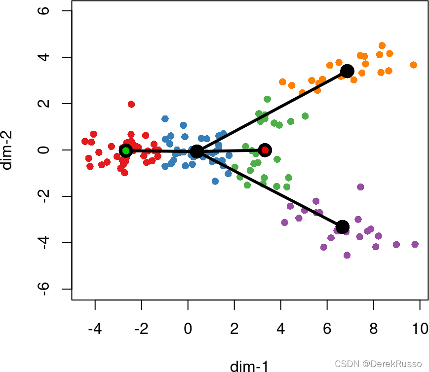

 

（2）constructing smooth curves and ordering cells

crv1 <- getCurves(lin1)
crv1

plot(rd, col = brewer.pal(9,"Set1")[cl], asp = 1, pch = 16)
lines(SlingshotDataSet(crv1), lwd = 3, col = 'black')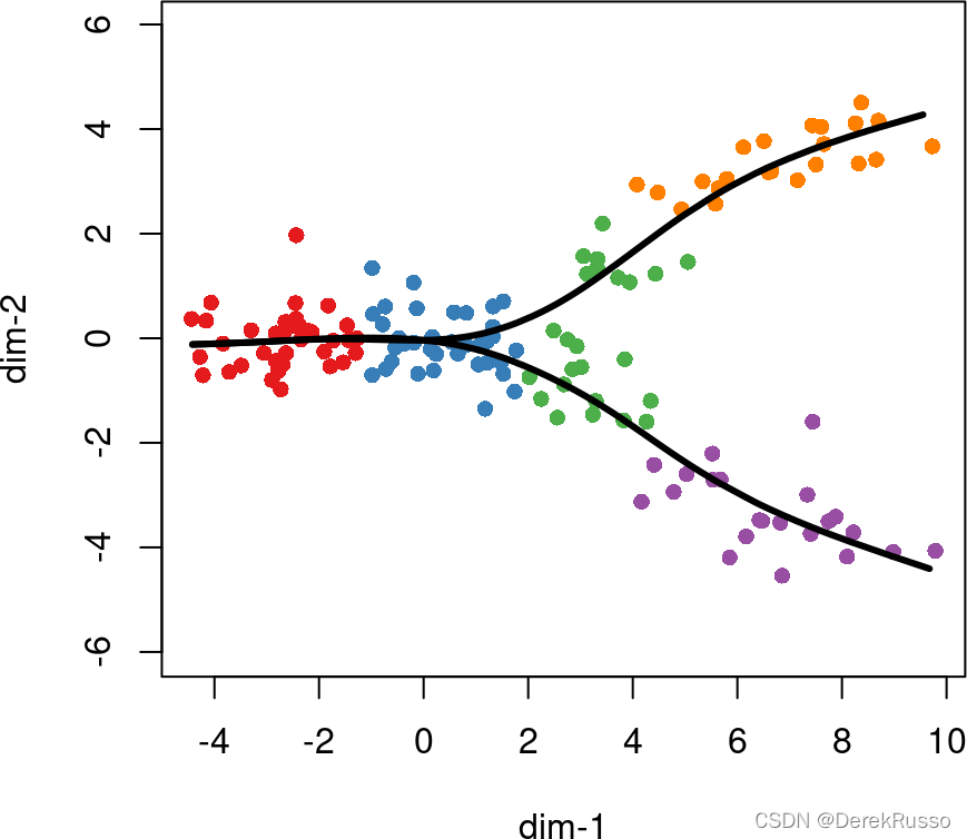

（3）running slingshot on large datasets

在slingshot或者getCurves功能中，可以用approx_points参数去调节projection resolution.官方推荐100-200之间，默认150.如果设置approx_points = F，则有多少细胞便会投影出多少个点，计算量也非常的大。