


今天介绍下遗传算法,在你以后的论文写作中可以水一节,胆子大的人才可以水一章
这些算法仅作为你的了解,不需要开始学习,如果以后需要在论文中用到,在针对性的了解下处理逻辑。
下面介绍这几种常见的优化算法
- 遗传算法GA
- 粒子群优化PSO
- 模拟退火SA
一、列表推导式
今天的代码用到了这个知识点,这是python里面的一个语法糖,我本来学习一下
列表推导式是 Python 中用于快速生成列表的语法结构,它以简洁的方式替代了 “创建空列表 + for 循环 + 条件判断(可选)” 的繁琐流程,让代码更紧凑、可读性更强。
语法糖是指 “对功能没有本质改变,但让代码更简洁、易读的语法形式”。列表推导式本质上可以被等价的 for 循环替代,但写法更优雅。
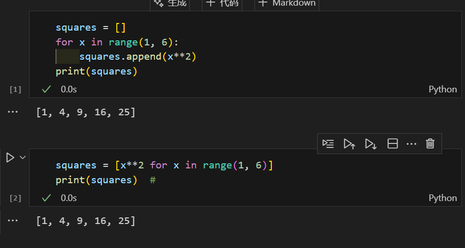
1.1 简单的列表推导式
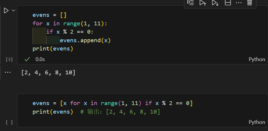
1.2 带条件过滤的列表推导式
生成 1 到 10 中所有偶数的列表。
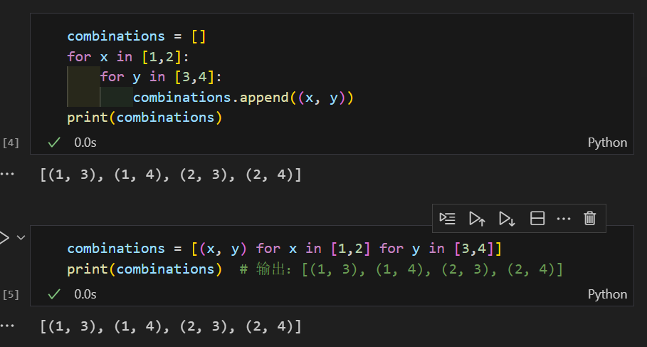
1.3 带嵌套循环的列表推导式
生成两个列表 [1,2] 和 [3,4] 的所有元素组合(笛卡尔积)。
笛卡尔积(Cartesian Product)是数学和计算机科学中一个基础概念,简单来说,它是两个或多个集合中所有可能的元素组合。
设有集合 A = {1, 2},集合 B = {3, 4},它们的笛卡尔积就是所有以 A 中元素为第一个元素、B 中元素为第二个元素的有序对,即:
A × B = {(1, 3), (1, 4), (2, 3), (2, 4)}
在编程中,笛卡尔积常用来生成 “所有可能的组合”。比如:
- 两个列表 [a, b] 和 [x, y] 的笛卡尔积是 [(a,x), (a,y), (b,x), (b,y)]
- 三个集合的笛卡尔积则是所有三元组的组合(如 A×B×C 的元素是 (a,b,c),其中 a∈A、b∈B、c∈C)
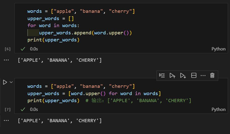
1.4 结合函数调用
对一个字符串列表,每个元素都调用 upper() 方法转为大写
二、启发式算法
2.1 前置工作
# 先运行之前预处理好的代码
import pandas as pd
import pandas as pd    #用于数据处理和分析,可处理表格数据。
import numpy as np     #用于数值计算,提供了高效的数组操作。
import matplotlib.pyplot as plt    #用于绘制各种类型的图表
import seaborn as sns   #基于matplotlib的高级绘图库,能绘制更美观的统计图形。
import warnings
warnings.filterwarnings('ignore')  #忽略警告信息,保持输出清洁。

 # 设置中文字体(解决中文显示问题)
plt.rcParams['font.sans-serif'] = ['SimHei']  # Windows系统常用黑体字体
plt.rcParams['axes.unicode_minus'] = False    # 正常显示负号
data = pd.read_csv('E:\study\PythonStudy\python60-days-challenge-master\data.csv')    #读取数据

# 先筛选字符串变量
discrete_features = data.select_dtypes(include=['object']).columns.tolist()
# Home Ownership 标签编码
home_ownership_mapping = {
    'Own Home': 1,
    'Rent': 2,
    'Have Mortgage': 3,
    'Home Mortgage': 4
}
data['Home Ownership'] = data['Home Ownership'].map(home_ownership_mapping)

# Years in current job 标签编码
years_in_job_mapping = {
    '< 1 year': 1,
    '1 year': 2,
    '2 years': 3,
    '3 years': 4,
    '4 years': 5,
    '5 years': 6,
    '6 years': 7,
    '7 years': 8,
    '8 years': 9,
    '9 years': 10,
    '10+ years': 11
}
data['Years in current job'] = data['Years in current job'].map(years_in_job_mapping)

# Purpose 独热编码,记得需要将bool类型转换为数值
data = pd.get_dummies(data, columns=['Purpose'])
data2 = pd.read_csv("E:\study\PythonStudy\python60-days-challenge-master\data.csv") # 重新读取数据,用来做列名对比
list_final = [] # 新建一个空列表,用于存放独热编码后新增的特征名
for i in data.columns:
    if i not in data2.columns:
       list_final.append(i) # 这里打印出来的就是独热编码后的特征名
for i in list_final:
    data[i] = data[i].astype(int) # 这里的i就是独热编码后的特征名


# Term 0 - 1 映射
term_mapping = {
    'Short Term': 0,
    'Long Term': 1
}
data['Term'] = data['Term'].map(term_mapping)
data.rename(columns={'Term': 'Long Term'}, inplace=True) # 重命名列
continuous_features = data.select_dtypes(include=['int64', 'float64']).columns.tolist()  #把筛选出来的列名转换成列表

 # 连续特征用中位数补全
for feature in continuous_features:
    mode_value = data[feature].mode()[0]            #获取该列的众数。
    data[feature].fillna(mode_value, inplace=True)          #用众数填充该列的缺失值,inplace=True表示直接在原数据上修改。

# 最开始也说了 很多调参函数自带交叉验证,甚至是必选的参数,你如果想要不交叉反而实现起来会麻烦很多
# 所以这里我们还是只划分一次数据集
from sklearn.model_selection import train_test_split
X = data.drop(['Credit Default'], axis=1)  # 特征,axis=1表示按列删除
y = data['Credit Default'] # 标签
# 按照8:2划分训练集和测试集
X_train, X_test, y_train, y_test = train_test_split(X, y, test_size=0.2, random_state=42)  # 80%训练集,20%测试集
from sklearn.ensemble import RandomForestClassifier #随机森林分类器
from sklearn.metrics import accuracy_score, precision_score, recall_score, f1_score # 用于评估分类器性能的指标
from sklearn.metrics import classification_report, confusion_matrix #用于生成分类报告和混淆矩阵
import warnings #用于忽略警告信息
warnings.filterwarnings("ignore") # 忽略所有警告信息
# --- 1. 默认参数的随机森林 ---
# 评估基准模型,这里确实不需要验证集
print("--- 1. 默认参数随机森林 (训练集 -> 测试集) ---")
import time # 这里介绍一个新的库,time库,主要用于时间相关的操作,因为调参需要很长时间,记录下会帮助后人知道大概的时长
start_time = time.time() # 记录开始时间
rf_model = RandomForestClassifier(random_state=42)
rf_model.fit(X_train, y_train) # 在训练集上训练
rf_pred = rf_model.predict(X_test) # 在测试集上预测
end_time = time.time() # 记录结束时间
print(f"训练与预测耗时: {end_time - start_time:.4f} 秒")
print("\n默认随机森林 在测试集上的分类报告:")
print(classification_report(y_test, rf_pred))
print("默认随机森林 在测试集上的混淆矩阵:")
print(confusion_matrix(y_test, rf_pred))核心思想:
- 这些启发式算法都是优化器。你的目标是找到一组超参数,让你的机器学习模型在某个指标(比如验证集准确率)上表现最好。
- 这个过程就像在一个复杂的地形(参数空间)上寻找最高峰(最佳性能)。
- 启发式算法就是一群聪明的“探险家”,它们用不同的策略(模仿自然、物理现象等)来寻找这个最高峰,而不需要知道地形每一处的精确梯度(导数)。
2.2 遗传算法
遗传算法 (Genetic Algorithm - GA)
- 灵感来源: 生物进化,达尔文的“适者生存”。
- 简单理解: 把不同的超参数组合想象成一群“个体”。表现好的个体(高验证分)更有机会“繁殖”(它们的参数组合会被借鉴和混合),并可能发生“变异”(参数随机小改动),产生下一代。表现差的个体逐渐被淘汰。一代代下去,种群整体就会越来越适应环境(找到更好的超参数)。
- 应用感觉: 像是在大范围“撒网”搜索,通过优胜劣汰和随机变动逐步逼近最优解。适合参数空间很大、很复杂的情况。

In [3]:
# pip install deap -i https://pypi.tuna.tsinghua.edu.cn/simple
DEAP 是一个非常著名的 Python 进化计算(Evolutionary Computation, EC)框架。全称是 Distributed Evolutionary Algorithms in Python(Python 分布式进化算法),DEAP 的设计理念是追求算法的显式化和数据结构的透明化,与其他许多将算法封装成“黑箱”的库不同,DEAP 鼓励用户清楚地理解和自定义进化过程中的每一个步骤。
除了能够实现今天要说的这些单目标优化算法外,还可以实现多目标优化算法。
from sklearn.ensemble import RandomForestClassifier
from sklearn.metrics import accuracy_score, precision_score, recall_score, f1_score
from sklearn.metrics import classification_report, confusion_matrix
import warnings
warnings.filterwarnings("ignore")
import time
from deap import base, creator, tools, algorithms # DEAP是一个用于遗传算法和进化计算的Python库
import random
import numpy as np

# --- 2. 遗传算法优化随机森林 ---
print("\n--- 2. 遗传算法优化随机森林 (训练集 -> 测试集) ---")

# 定义适应度函数和个体类型
creator.create("FitnessMax", base.Fitness, weights=(1.0,))
creator.create("Individual", list, fitness=creator.FitnessMax)

# 定义超参数范围
n_estimators_range = (50, 200)
max_depth_range = (10, 30)
min_samples_split_range = (2, 10)
min_samples_leaf_range = (1, 4)

# 初始化工具盒
toolbox = base.Toolbox()

# 定义基因生成器,随机生成超参数值。注册这个操作是为了让代码更加模块化和可重用。
toolbox.register("attr_n_estimators", random.randint, *n_estimators_range) # 随机生成n_estimators的值
toolbox.register("attr_max_depth", random.randint, *max_depth_range)
toolbox.register("attr_min_samples_split", random.randint, *min_samples_split_range)
toolbox.register("attr_min_samples_leaf", random.randint, *min_samples_leaf_range)

# 定义个体生成器,将各基因组合成个体
toolbox.register("individual", tools.initCycle, creator.Individual,
                 (toolbox.attr_n_estimators, toolbox.attr_max_depth,
                  toolbox.attr_min_samples_split, toolbox.attr_min_samples_leaf), n=1)

# 定义种群生成器,将个体组合成种群
toolbox.register("population", tools.initRepeat, list, toolbox.individual)

# 定义评估函数,计算个体的适应度(准确率)
def evaluate(individual):
    n_estimators, max_depth, min_samples_split, min_samples_leaf = individual
    model = RandomForestClassifier(n_estimators=n_estimators,
                                   max_depth=max_depth,
                                   min_samples_split=min_samples_split,
                                   min_samples_leaf=min_samples_leaf,
                                   random_state=42)
    model.fit(X_train, y_train)
    y_pred = model.predict(X_test)
    accuracy = accuracy_score(y_test, y_pred)
    return accuracy,

# 注册评估函数
toolbox.register("evaluate", evaluate)

# 注册遗传操作,交叉和变异
toolbox.register("mate", tools.cxTwoPoint)
toolbox.register("mutate", tools.mutUniformInt, low=[n_estimators_range[0], max_depth_range[0],
                                                     min_samples_split_range[0], min_samples_leaf_range[0]],
                 up=[n_estimators_range[1], max_depth_range[1],
                     min_samples_split_range[1], min_samples_leaf_range[1]], indpb=0.1)
toolbox.register("select", tools.selTournament, tournsize=3)

# 初始化种群
pop = toolbox.population(n=20)

# 遗传算法参数
NGEN = 10  # 迭代代数
CXPB = 0.5 # 交叉概率
MUTPB = 0.2 # 变异概率

start_time = time.time()
# 运行遗传算法
for gen in range(NGEN): # 迭代NGEN代
    offspring = algorithms.varAnd(pop, toolbox, cxpb=CXPB, mutpb=MUTPB) # 变异和交叉生成后代
    fits = toolbox.map(toolbox.evaluate, offspring) # 评估后代适应度
    for fit, ind in zip(fits, offspring): # 更新个体适应度
        ind.fitness.values = fit # 更新个体的适应度值
    pop = toolbox.select(offspring, k=len(pop)) # 选择下一代种群

end_time = time.time()

# 找到最优个体
best_ind = tools.selBest(pop, k=1)[0] # 选择适应度最高的个体
best_n_estimators, best_max_depth, best_min_samples_split, best_min_samples_leaf = best_ind # 解包最佳参数

print(f"遗传算法优化耗时: {end_time - start_time:.4f} 秒")
print("最佳参数: ", {
    'n_estimators': best_n_estimators,
    'max_depth': best_max_depth,
    'min_samples_split': best_min_samples_split,
    'min_samples_leaf': best_min_samples_leaf
})

# 使用最佳参数的模型进行预测
best_model = RandomForestClassifier(n_estimators=best_n_estimators,
                                    max_depth=best_max_depth,
                                    min_samples_split=best_min_samples_split,
                                    min_samples_leaf=best_min_samples_leaf,
                                    random_state=42)
best_model.fit(X_train, y_train)
best_pred = best_model.predict(X_test)

print("\n遗传算法优化后的随机森林 在测试集上的分类报告:")
print(classification_report(y_test, best_pred))
print("遗传算法优化后的随机森林 在测试集上的混淆矩阵:")
print(confusion_matrix(y_test, best_pred))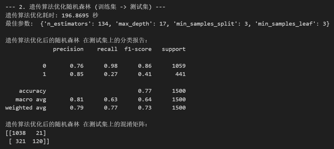
上述代码看上去非常复杂,而且不具备复用性
也就是说,即使你搞懂了这段代码,对你的提升也微乎其微,因为你无法对他进行改进(他永远是别人的东西),而且就算背熟悉了他,也对你学习其他的方法没什么帮助,即使你学完遗传算法学粒子群,也没有帮助。
AI时代的工具很大的好处,就是找到了一个记忆工具来帮助我们记住这个方法需要的步骤,然后我们只需要调用这个工具,就可以完成这个任务。
- 关注输入和输出的格式和数据
- 关注方法的前生今世和各自的优势---优缺点和应用场景
- 关注模型本身的实现逻辑(如果用的时候很少,可跳过,借助ai实现)
2.3 粒子群方法

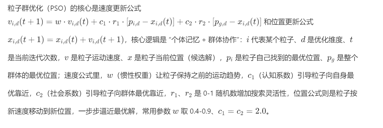
粒子群优化 (Particle Swarm Optimization - PSO)
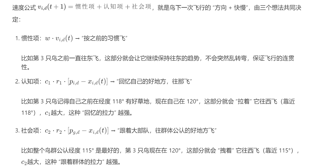
- 灵感来源: 鸟群或鱼群觅食。
- 简单理解: 把每个超参数组合想象成一个“粒子”(鸟)。每个粒子在参数空间中“飞行”。它会记住自己飞过的最好位置,也会参考整个“鸟群”发现的最好位置,结合这两者来调整自己的飞行方向和速度,同时带点随机性。
- 应用感觉: 像是一群探险家,既有自己的探索记忆,也会互相交流信息(全局最佳位置),集体协作寻找目标。通常收敛比遗传算法快一些。
粒子群方法的思想比较简单,所以甚至可以不调库自己实现。
# --- 2. 粒子群优化算法优化随机森林 ---
print("\n--- 2. 粒子群优化算法优化随机森林 (训练集 -> 测试集) ---")


# 定义适应度函数,本质就是构建了一个函数实现 参数--> 评估指标的映射
def fitness_function(params):
    n_estimators, max_depth, min_samples_split, min_samples_leaf = params # 序列解包,允许你将一个可迭代对象(如列表、元组、字符串等)中的元素依次赋值给多个变量。
    model = RandomForestClassifier(n_estimators=int(n_estimators),
                                   max_depth=int(max_depth),
                                   min_samples_split=int(min_samples_split),
                                   min_samples_leaf=int(min_samples_leaf),
                                   random_state=42)
    model.fit(X_train, y_train)
    y_pred = model.predict(X_test)
    accuracy = accuracy_score(y_test, y_pred)
    return accuracy


# 粒子群优化算法实现
def pso(num_particles, num_iterations, c1, c2, w, bounds): # 粒子群优化算法核心函数
    # num_particles:粒子的数量,即算法中用于搜索最优解的个体数量。
    # num_iterations:迭代次数,算法运行的最大循环次数。
    # c1:认知学习因子,用于控制粒子向自身历史最佳位置移动的程度。
    # c2:社会学习因子,用于控制粒子向全局最佳位置移动的程度。
    # w:惯性权重,控制粒子的惯性,影响粒子在搜索空间中的移动速度和方向。
    # bounds:超参数的取值范围,是一个包含多个元组的列表,每个元组表示一个超参数的最小值和最大值。

    num_params = len(bounds)  # 超参数的数量
    particles = np.array([[random.uniform(bounds[i][0], bounds[i][1]) for i in range(num_params)] for _ in
                          range(num_particles)]) # 初始化粒子位置,外层管粒子数,内层管参数数
    velocities = np.array([[0] * num_params for _ in range(num_particles)]) # 初始化速度为0
    personal_best = particles.copy() # 每个粒子的历史最佳位置
    personal_best_fitness = np.array([fitness_function(p) for p in particles]) # 每个粒子的历史最佳适应度
    global_best_index = np.argmax(personal_best_fitness) # 全局最佳粒子索引
    global_best = personal_best[global_best_index] # 全局最佳位置
    global_best_fitness = personal_best_fitness[global_best_index] # 全局最佳适应度

    for _ in range(num_iterations): # 迭代更新粒子位置和速度
        r1 = np.array([[random.random() for _ in range(num_params)] for _ in range(num_particles)]) # 生成随机数矩阵
        r2 = np.array([[random.random() for _ in range(num_params)] for _ in range(num_particles)]) # 生成随机数矩阵

        velocities = w * velocities + c1 * r1 * (personal_best - particles) + c2 * r2 * (
                global_best - particles) # 更新速度
        particles = particles + velocities # 更新位置

        for i in range(num_particles): # 保持粒子在边界内
            for j in range(num_params): # 遍历每个参数
                if particles[i][j] < bounds[j][0]: # 下界
                    particles[i][j] = bounds[j][0] # 下界处理
                elif particles[i][j] > bounds[j][1]: # 上界
                    particles[i][j] = bounds[j][1] # 上界处理

        fitness_values = np.array([fitness_function(p) for p in particles]) # 计算适应度
        improved_indices = fitness_values > personal_best_fitness # 找到适应度提升的粒子索引
        personal_best[improved_indices] = particles[improved_indices] # 更新历史最佳位置
        personal_best_fitness[improved_indices] = fitness_values[improved_indices] # 更新历史最佳适应度

        current_best_index = np.argmax(personal_best_fitness) # 当前全局最佳粒子索引
        if personal_best_fitness[current_best_index] > global_best_fitness: # 更新全局最佳位置和适应度
            global_best = personal_best[current_best_index] # 全局最佳位置
            global_best_fitness = personal_best_fitness[current_best_index] # 全局最佳适应度

    return global_best, global_best_fitness # 返回全局最佳位置和适应度


# 超参数范围
bounds = [(50, 200), (10, 30), (2, 10), (1, 4)]  # n_estimators, max_depth, min_samples_split, min_samples_leaf

# 粒子群优化算法参数
num_particles = 20
num_iterations = 10
c1 = 1.5
c2 = 1.5
w = 0.5

start_time = time.time()
best_params, best_fitness = pso(num_particles, num_iterations, c1, c2, w, bounds)
end_time = time.time()

print(f"粒子群优化算法优化耗时: {end_time - start_time:.4f} 秒")
print("最佳参数: ", {
    'n_estimators': int(best_params[0]),
   'max_depth': int(best_params[1]),
   'min_samples_split': int(best_params[2]),
   'min_samples_leaf': int(best_params[3])
})

# 使用最佳参数的模型进行预测
best_model = RandomForestClassifier(n_estimators=int(best_params[0]),
                                    max_depth=int(best_params[1]),
                                    min_samples_split=int(best_params[2]),
                                    min_samples_leaf=int(best_params[3]),
                                    random_state=42)
best_model.fit(X_train, y_train)
best_pred = best_model.predict(X_test)

print("\n粒子群优化算法优化后的随机森林 在测试集上的分类报告:")
print(classification_report(y_test, best_pred))
print("粒子群优化算法优化后的随机森林 在测试集上的混淆矩阵:")
print(confusion_matrix(y_test, best_pred))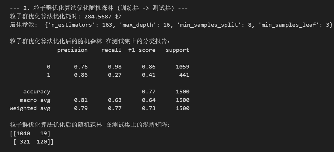
2.4 退火算法
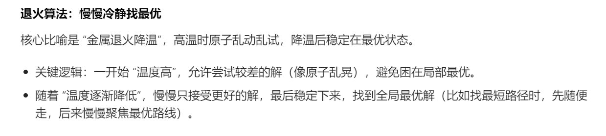
模拟退火 (Simulated Annealing - SA)
- 灵感来源: 金属冶炼中的退火过程(缓慢冷却使金属达到最低能量稳定态)。
- 简单理解: 从一个随机的超参数组合开始。随机尝试改变一点参数。如果新组合更好,就接受它。如果新组合更差,也有一定概率接受它(尤其是在“高温”/搜索早期)。这个接受坏解的概率会随着时间(“降温”)慢慢变小。
- 应用感觉: 像一个有点“冲动”的探险家,初期愿意尝试一些看起来不太好的路径(为了跳出局部最优的小山谷),后期则越来越“保守”,专注于在当前找到的好区域附近精细搜索。擅长避免陷入局部最优。
# --- 2. 模拟退火算法优化随机森林 ---
print("\n--- 2. 模拟退火算法优化随机森林 (训练集 -> 测试集) ---")


# 定义适应度函数
def fitness_function(params):
    n_estimators, max_depth, min_samples_split, min_samples_leaf = params
    model = RandomForestClassifier(n_estimators=int(n_estimators),
                                   max_depth=int(max_depth),
                                   min_samples_split=int(min_samples_split),
                                   min_samples_leaf=int(min_samples_leaf),
                                   random_state=42)
    model.fit(X_train, y_train)
    y_pred = model.predict(X_test)
    accuracy = accuracy_score(y_test, y_pred)
    return accuracy


# 模拟退火算法实现
def simulated_annealing(initial_solution, bounds, initial_temp, final_temp, alpha):
    current_solution = initial_solution
    current_fitness = fitness_function(current_solution)
    best_solution = current_solution
    best_fitness = current_fitness
    temp = initial_temp

    while temp > final_temp:
        # 生成邻域解
        neighbor_solution = []
        for i in range(len(current_solution)):
            new_val = current_solution[i] + random.uniform(-1, 1) * (bounds[i][1] - bounds[i][0]) * 0.1
            new_val = max(bounds[i][0], min(bounds[i][1], new_val))
            neighbor_solution.append(new_val)

        neighbor_fitness = fitness_function(neighbor_solution)
        delta_fitness = neighbor_fitness - current_fitness

        if delta_fitness > 0 or random.random() < np.exp(delta_fitness / temp):
            current_solution = neighbor_solution
            current_fitness = neighbor_fitness

        if current_fitness > best_fitness:
            best_solution = current_solution
            best_fitness = current_fitness

        temp *= alpha

    return best_solution, best_fitness


# 超参数范围
bounds = [(50, 200), (10, 30), (2, 10), (1, 4)]  # n_estimators, max_depth, min_samples_split, min_samples_leaf

# 模拟退火算法参数
initial_temp = 100 # 初始温度
final_temp = 0.1 # 终止温度
alpha = 0.95 # 温度衰减系数

# 初始化初始解
initial_solution = [random.uniform(bounds[i][0], bounds[i][1]) for i in range(len(bounds))]

start_time = time.time()
best_params, best_fitness = simulated_annealing(initial_solution, bounds, initial_temp, final_temp, alpha)
end_time = time.time()

print(f"模拟退火算法优化耗时: {end_time - start_time:.4f} 秒")
print("最佳参数: ", {
    'n_estimators': int(best_params[0]),
    'max_depth': int(best_params[1]),
    'min_samples_split': int(best_params[2]),
    'min_samples_leaf': int(best_params[3])
})

# 使用最佳参数的模型进行预测
best_model = RandomForestClassifier(n_estimators=int(best_params[0]),
                                    max_depth=int(best_params[1]),
                                    min_samples_split=int(best_params[2]),
                                    min_samples_leaf=int(best_params[3]),
                                    random_state=42)
best_model.fit(X_train, y_train)
best_pred = best_model.predict(X_test)

print("\n模拟退火算法优化后的随机森林 在测试集上的分类报告:")
print(classification_report(y_test, best_pred))
print("模拟退火算法优化后的随机森林 在测试集上的混淆矩阵:")
print(confusion_matrix(y_test, best_pred))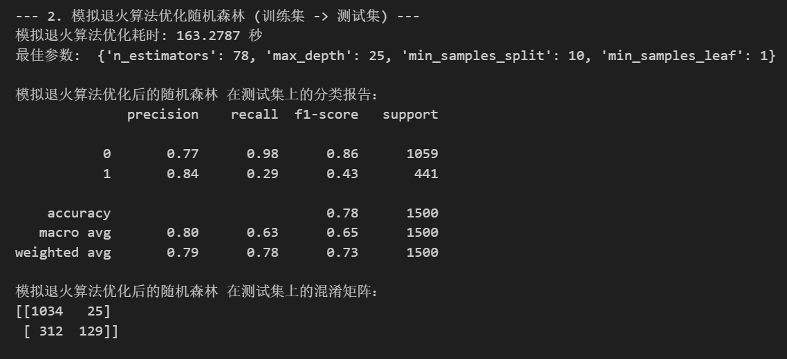


 3万+
3万+

 被折叠的 条评论
为什么被折叠?
被折叠的 条评论
为什么被折叠?
 到【灌水乐园】发言


