深度学习基础篇（一）

学习来源：PyTorch深度学习简明实战（日月光华 /著）

相比较于tensorflow，pytorch可以不用依赖cuDNN，环境配置相对较少，但是tensorflow可以在多个平台上运行。

1.GPU版本PyTorch安装

环境搭建：略
pip install torch torchvision
hello world测试：

import torch

# 生成矩阵（自动分配到GPU）
matrix = torch.rand(99, 99).cuda()

# 计算平方（GPU加速）
squared_matrix = matrix ** 2

# 输出结果
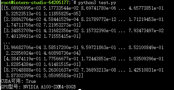
print(squared_matrix.cpu().numpy())  # 转回CPU内存

# import torch
print("CUDA可用:", torch.cuda.is_available())
if torch.cuda.is_available():
    print("GPU型号:", torch.cuda.get_device_name(0))

jupyterNotebook测试：

!pip install numpy
!pip install matplotlib
import numpy as np
import matplotlib.pyplot as plt

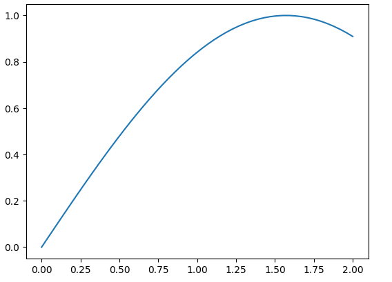
x = np.linspace(0,2)
y = np.sin(x)
plt.plot(x,y)
plt.show()

demo案例；

import torch

#随机初始化张量
x = torch.rand(5,3)
print(x)

# 判断是否启动了CUDA驱动程序
print(torch.cuda.is_available())

2.机器学习基础与线性回归

2.1机器学习基础

模型学习基本过程：
1.创建模型
2.输入一张带标签的图片
3.使用模型对此图片做出预测
4.将预测结果与实际结果标签比较，产生的差距一般称为损失
5.以减小损失为优化目标，根据损失优化模型参数
6.循环重复上述第2-5步骤

2.2线性回归

income.csv

education,income
10,26.658839
10.401338,27.306435
10.842809,22.132410
9.5,24.87
10.2,26.12
11.1,28.95
10.9,27.43
11.5,30.11
9.8,25.34
10.6,26.89
11.3,29.27
10.1,25.98
11.7,30.56

CPU版本:

import torch
import pandas as pd
import numpy as np
import matplotlib.pyplot as plt

data = pd.read_csv('dataset/income.csv')
print(data.head(3)) #打印前三行
print(data.info()) #查看数据整体情况

plt.scatter(data.education,data.income) #绘制散点图
plt.xlabel('edccation')
plt.ylabel('income')
plt.show()
plt.savefig('scatter_plot.png') #保存为png图片

# 在一元线性回归之中，y = ax+b,a,b是常数，x是变量输入，y是输出
# 我们用y表示income，x表示education
X = torch.from_numpy(data.education.to_numpy().reshape(-1,1)).type(torch.FloatTensor) #首先通过data.education获取教育这一列，然后将其转换成ndarray数组形式，然后reshape成为二维数组，并将最后一个维度明确为1
Y = torch.from_numpy(data.income.to_numpy().reshape(-1,1)).type(torch.FloatTensor)
# 打印形状
print(X.size(),Y.size()) #torch.Size([13, 1]) torch.Size([13, 1])

# 定义模型EI--education-income模型
from torch import nn
class EIModel(nn.Module):
    def __init__(self):
        super(EIModel,self).__init__() #继承父类属性
        self.linear = nn.Linear(in_features=1,out_features=1) #创建线性层
    def forward(self,inputs):
        logits = self.linear(inputs) #在输入上调用初始化的线性层
        return logits

# 初始化实例
model= EIModel()
loss_fn = nn.MSELoss() #定义均方误差损失计算函数
opt = torch.optim.SGD(model.parameters(),lr=0.0001) #初始化优化器,lr代表学习速率

# 训练循环代码，在这里对全部数据训练5000次，每一次循环中执行以下操作：
# 1.调用模型获取预测
# 2.根据预测计算损失
# 3.根据损失优化模型参数
 
for epoch in range(5000): #对全部数据训练5000次
    for x,y in zip(X,Y): #同时对X和Y进行迭代
        y_pred = model(x) #调整model得到预测输出y_pred
        loss = loss_fn(y_pred,y)