可以做structure的R语言包：LEA

1. paper

LEA: An R package for landscape and ecological association studies

使用说明文档

不同格式的数据使用LEA

2. 软件介绍

This short tutorial explains how population structure analyses reproducing the results of the widely-used computer program structure can be performed using commands in the R language. The method works for any operating systems, and it does not require the installation
of structure or additional computer programs. The R program allows running population structure inference algorithms, choosing the number of clusters, and showing admixture coefficient bar-plots using a few commands. The methods used by R are fast and accurate, and they
are free of standard population genetic equilibrium hypotheses. In addition, these methods allow their users to play with a large panel of graphical functions for displaying pie-charts and interpolated admixture coefficients on geographic maps.

划重点:

• 可以在R语言中实现软件Structure的功能
• 可以做类似admixture的图
• 简单操作, 几个命令实现相关功能
• C语言开发, 可以处理大数据

3. 软件安装

install.packages(c("fields","RColorBrewer","mapplots"))
source("http://bioconductor.org/biocLite.R")
biocLite("LEA")

如果安装不成功, 也可以通过CRAN把软件包下载到本地, 进行安装:

install.packages("LEA_1.4.0_tar.gz", repos = NULL, type ="source")

载入两个函数, 进行格式转化以及可视化:

source("http://membres-timc.imag.fr/Olivier.Francois/Conversion.R")
source("http://membres-timc.imag.fr/Olivier.Francois/POPSutilities.R")

4. 测试数据

plink格式的ped文件, 具体格式参考:plink格式的ped和map文件及转化为012的方法

1 SAMPLE0 0 0 2 2 1 2 3 3 1 1 2 1
2 SAMPLE1 0 0 1 2 2 1 1 3 0 4 1 1
3 SAMPLE2 0 0 2 1 2 2 3 3 1 4 1 1

前六列为:
家系ID
个体ID
父本
母本
性别
表型值
SNP1-1(SNP1的第一个位点)
SNP1-2(SNP的第二个位点)

测试数据采用admixture的示例数据, 使用plink将其转化为ped文件

library(LEA)
# 结果会生成test.geno文件的数据.
output = ped2lfmm("test.ped")

# 使用LEA进行structure进行分析
library(LEA)
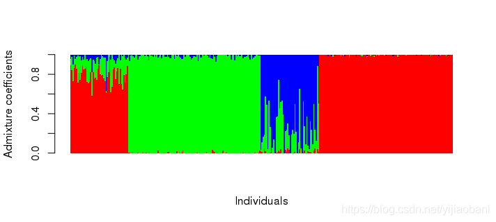
obj.snmf = snmf("test.geno", K = 3, alpha = 100, project = "new")
qmatrix = Q(obj.snmf, K = 3)
head(qmatrix)
barplot(t(qmatrix), col = rainbow(3), border = NA, space = 0,
        xlab = "Individuals", ylab = "Admixture coefficients")

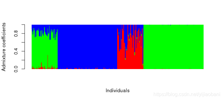
对比admixture的结果

# 对比admixture结果
qad = read.table("test.3.Q")
head(qad)
barplot(t(qad), col = rainbow(3), border = NA, space = 0,
        xlab = "Individuals", ylab = "Admixture coefficients")

5. 使用snmf选择最优K值

# 绘制折线图, 选择最优K值.
plot(project, col = "blue", pch = 19, cex = 1.2)

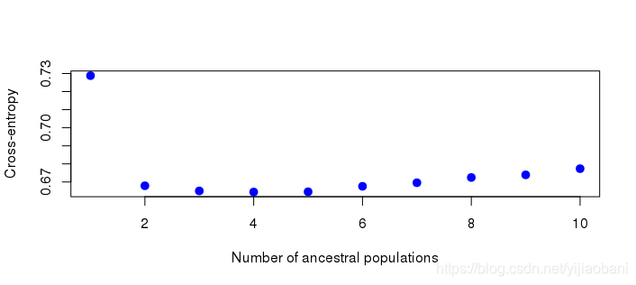
可以看出, K=3时, 最小, 因此选择K=3.