图的宽度优先搜索和最短路径实现——python

最新推荐文章于 2025-06-11 20:08:26 发布

woshilsh

最新推荐文章于 2025-06-11 20:08:26 发布

阅读量1.5k

点赞数 1

CC 4.0 BY-SA版权

分类专栏：作业题

本文链接：https://blog.youkuaiyun.com/woshilsh/article/details/90207292

本文不记录课本上的手动实现，而是利用Python的网络分析库和绘图库来演示宽度优先搜索（BFS）和最短路径的求解。通过代码展示如何构造图，并解释了输出结果，包括宽度优先搜索的节点顺序和所有从源点出发的最短路径。虽然库函数的编写较为复杂，但考虑周全，值得学习。

摘要生成于 C知道，由 DeepSeek-R1 满血版支持，前往体验 >

课本上的是手动造轮子，尽管不完善，但是挺好用。这里就不记录课本上的了，通俗易懂，我们主要看看用库函数实现课本上的这俩功能，开阔下思路。
主要用到了网络分析库和绘图库，看代码：

import networkx as nx
import matplotlib.pyplot as plt

G = nx.Graph()
nodes = ['s', 'a', 'z', 'x', 'd', 'c', 'f', 'v']
G.add_nodes_from(nodes)
ebunch = [('a', 'z'), ('a', 's'), ('s', 'x'), ('x', 'd'),
          ('d', 'c'), ('x', 'c'), ('d', 'f'), ('c', 'f'),
          ('c', 'v'), ('f', 'v')]
G.add_edges_from(ebunch)
nx.draw(G, pos=nx.spring_layout(G), with_labels=True, font_size=24, node_size=2640)
plt.show()
print(nx.bfs_predecessors(G, 's'))
print(nx.shortest_path(G, 's'))

打印出来的结果，看下图和课本图7.4即可，我们这里稍微解释下输出，和课本上的类似：

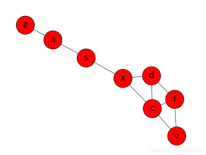
{'a': 's', 'c': 'x', 'd': 'x', 'f': 'c', 'v': 'c', 'x': 's', 'z': 'a'}
{'a': ['s', 'a'], 'c': ['s', 'x', 'c'], 'd': ['s', 'x', 'd'], 'f': ['s', 'x', 'c', 'f'], 's': ['s'], 'v': ['s'