第四章.误差反向传播法—误差反向传播法实现手写数字识别神经网络

第四章.误差反向传播法

4.3 误差反向传播法实现手写数字识别神经网络

通过像组装乐高积木一样组装第四章中实现的层，来构建神经网络。

1.神经网络学习全貌图

1).前提：

• 神经网络存在合适的权重和偏置，调整权重和偏置以便拟合训练数据的过程称为“学习”，神经网络的学习分成下面4个步骤。

2).步骤1 (mini-batch):

• 从训练数据中随机选出一部分数据，这部分数据称为mini-batch,我们的目标是减少mini-batch损失函数的值。

3).步骤2 (计算梯度):

• 为了减少mini_batch损失函数的值，需要求出各个权重参数的梯度，梯度表示损失函数的值减少最多的方向。

4).步骤3 (更新参数):

• 将权重参数沿梯度方向进行微小更新

5).步骤4 (重复)：

• 重复步骤1，步骤2，步骤3

2.手写数字识别神经网络的实现:(2层)

# 误差反向传播法实现手写数字识别神经网络

import numpy as np
import matplotlib.pyplot as plt
import sys, os

sys.path.append(os.pardir)
from dataset.mnist import load_mnist
from collections import OrderedDict


class Affine:
    def __init__(self, W, b):
        self.W = W
        self.b = b
        self.x = None
        self.original_x_shape = None
        # 权重和偏置参数的导数
        self.dW = None
        self.db = None

    # 向前传播
    def forward(self, x):
        self.original_x_shape = x.shape
        x = x.reshape(x.shape[0], -1)
        self.x = x
        out = np.dot(self.x, self.W) + self.b
        return out

    # 反向传播
    def backward(self, dout):
        dx = np.dot(dout, self.W.T)
        self.dW = np.dot(self.x.T, dout)
        self.db = np.sum(dout, axis=0)

        dx = dx.reshape(*self.original_x_shape)  # 还原输入数据的形状（对应张量）
        return dx


class ReLU:
    def __init__(self):
        self.mask = None

    def forward(self, x):
        self.mask = (x <= 0)
        out = x.copy()
        out[self.mask] = 0
        return out

    def backward(self, dout):
        dout[self.mask] = 0
        dx = dout
        return dx


class SoftmaxWithLoss:
    def __init__(self):
        self.loss = None
        self.y = None
        self.t = None

    # 输出层函数：softmax
    def softmax(self, x):
        if x.ndim == 2:
            x = x.T
            x = x - np.max(x, axis=0)
            y = np.exp(x) / np.sum(np.exp(x), axis=0)
            return y.T

        x = x - np.max(x)  # 溢出对策
        y = np.exp(x) / np.sum(np.exp(x))
        return y

    # 误差函数：交叉熵误差
    def cross_entropy_error(self, y, t):
        if y.ndim == 1:
            y = y.reshape(1, y.size)
            t = t.reshape(1, t.size)

        # 监督数据是one_hot_label的情况下，转换为正确解标签的索引
        if t.size == y.size:
            t = t.argmax(axis=1)

        batch_size = y.shape[0]
        return -np.sum(np.log(y[np.arange(batch_size), t] + 1e-7)) / batch_size

    def forward(self, x, t):
        self.t = t
        self.y = self.softmax(x)
        self.loss = self.cross_entropy_error(self.y, self.t)
        return self.loss

    def backward(self, dout=1):
        batch_size = self.t.shape[0]
        if self.t.size == self.y.size:
            dx = (self.y - self.t) / batch_size
        else:
            dx = self.y.copy()
            dx[np.arange(batch_size), self.t] -= 1
            dx = dx / batch_size

        return dx


class TwoLayerNet:

    # 初始化
    def __init__(self, input_size, hidden_size, output_size, weight_init_std=0.01):
        # 初始化权重
        self.params = {}
        self.params['W1'] = weight_init_std * np.random.randn(input_size, hidden_size)
        self.params['b1'] = np.zeros(hidden_size)
        self.params['W2'] = weight_init_std * np.random.randn(hidden_size, output_size)
        self.params['b2'] = np.zeros(output_size)

        # 生成层
        self.layers = OrderedDict()
        self.layers['Affine1'] = Affine(self.params['W1'], self.params['b1'])
        self.layers['ReLU'] = ReLU()
        self.layers['Affine2'] = Affine(self.params['W2'], self.params['b2'])
        self.lastLayer = SoftmaxWithLoss()

    def predict(self, x):
        for layer in self.layers.values():
            x = layer.forward(x)
        return x

    def loss(self, x, t):
        y = self.predict(x)
        loss = self.lastLayer.forward(y, t)
        return loss

    def accuracy(self, x, t):
        y = self.predict(x)
        y = np.argmax(y, axis=1)
        if t.ndim != 1: t = np.argmax(t, axis=1)
        accuracy = np.sum(y == t) / float(t.shape[0])
        return accuracy

    # 微分函数
    def numerical_gradient1(self, f, x):
        h = 1e-4
        grad = np.zeros_like(x)
        it = np.nditer(x, flags=['multi_index'], op_flags=['readwrite'])
        while not it.finished:
            idx = it.multi_index
            tmp_val = x[idx]
            x[idx] = float(tmp_val) + h
            fxh1 = f(x)  # f(x+h)

            x[idx] = tmp_val - h
            fxh2 = f(x)  # f(x-h)
            grad[idx] = (fxh1 - fxh2) / (2 * h)

            x[idx] = tmp_val  # 还原值
            it.iternext()

        return grad

    # 通过数值微分计算关于权重参数的梯度
    def numerical_gradient(self, x, t):
        loss_W = lambda W: self.loss(x, t)
        grad = {}
        grad['W1'] = self.numerical_gradient1(loss_W, self.params['W1'])
        grad['b1'] = self.numerical_gradient1(loss_W, self.params['b1'])
        grad['W2'] = self.numerical_gradient1(loss_W, self.params['W2'])
        grad['b2'] = self.numerical_gradient1(loss_W, self.params['b2'])

        return grad

    # 通过误差反向传播法计算权重参数的梯度误差
    def gradient(self, x, t):
        # 正向传播
        self.loss(x, t)

        # 反向传播
        dout = 1
        dout = self.lastLayer.backward(dout)
        layers = list(self.layers.values())
        layers.reverse()
        for layer in layers:
            dout = layer.backward(dout)

        # 设定
        grads = {}
        grads['W1'] = self.layers['Affine1'].dW
        grads['b1'] = self.layers['Affine1'].db
        grads['W2'] = self.layers['Affine2'].dW
        grads['b2'] = self.layers['Affine2'].db

        return grads


# 读入数据
def get_data():
    (x_train, t_train), (x_test, t_test) = load_mnist(normalize=True, one_hot_label=True)
    return (x_train, t_train), (x_test, t_test)


# 读入数据
(x_train, t_train), (x_test, t_test) = get_data()

network = TwoLayerNet(input_size=784, hidden_size=50, output_size=10)

iters_num = 10000
train_size = x_train.shape[0]
batch_size = 100
lr = 0.1
train_loss_list = []
train_acc_list = []
test_acc_list = []
iter_per_epoch = max(train_size / batch_size, 1)

for i in range(iters_num):
    batch_mask = np.random.choice(train_size, batch_size)
    x_batch = x_train[batch_mask]
    t_batch = t_train[batch_mask]

    # 通过误差反向传播法求梯度
    grad = network.gradient(x_batch, t_batch)

    # 更新
    for key in ('W1', 'b1', 'W2', 'b2'):
        network.params[key] -= lr * grad[key]

    loss = network.loss(x_batch, t_batch)
    train_loss_list.append(loss)

    if i % iter_per_epoch == 0:
        train_acc = network.accuracy(x_train, t_train)
        train_acc_list.append(train_acc)
        test_acc = network.accuracy(x_test, t_test)
        test_acc_list.append(test_acc)
        print('train_acc,test_acc|', str(train_acc) + ',' + str(test_acc))

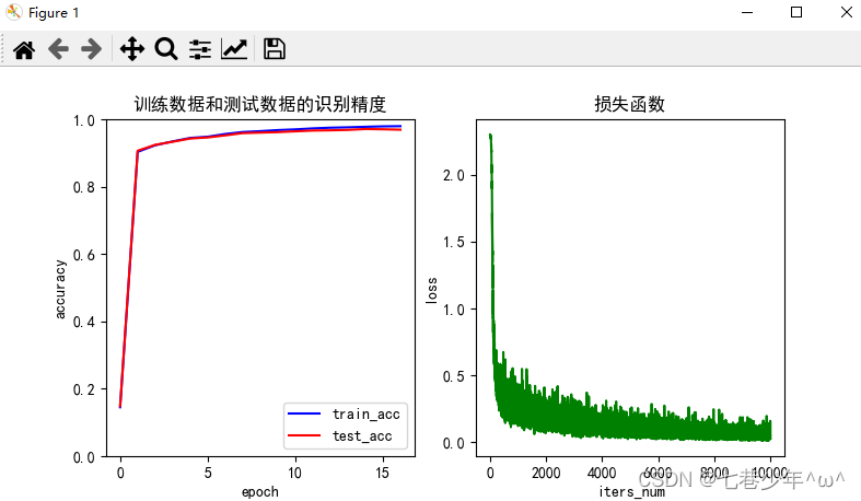
# 绘制识别精度图像
plt.rcParams['font.sans-serif'] = ['SimHei']  # 解决中文乱码
plt.rcParams['axes.unicode_minus'] = False  # 解决负号不显示的问题

plt.figure(figsize=(8, 4))
plt.subplot(1, 2, 1)
x_data = np.arange(0, len(train_acc_list))
plt.plot(x_data, train_acc_list, 'b')
plt.plot(x_data, test_acc_list, 'r')
plt.xlabel('epoch')
plt.ylabel('accuracy')
plt.ylim(0.0, 1.0)
plt.title('训练数据和测试数据的识别精度')
plt.legend(['train_acc', 'test_acc'])

plt.subplot(1, 2, 2)
x_data = np.arange(0, len(train_loss_list))
plt.plot(x_data, train_loss_list, 'g')
plt.xlabel('iters_num')
plt.ylabel('loss')
plt.title('损失函数')
plt.show()

3.结果展示