第三章.神经网络的学习—梯度,手写数字识别2层神经网络的实现

第三章.神经网络的学习

3.2 梯度

梯度法使用梯度的信息决定前进的方向，在介绍梯度法之前，先介绍一下导数和偏导。

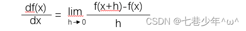
1.导数

1).公式：

2).代码实现：

• 注意：

  ①.h = 1e-4不可以使用过小的值，会出现计算出错的问题，例如：h = 1e-50 , result = 0.0

  ②.计算函数f(x)在x与x+h之间的差分，这个计算从一开始就有误差，“真的导数”对应函数在x处的斜率，但是上述公式中计算的导数对应的是x和(h+x)之间的斜率,因此，真的导数(“真的切线”)和上述公式中得到的导数值 在严格意义上是一致的，这个差异的出现是因为h不可能无限接近0。
  
  ③.为了减少这个误差，我们可以计算函数f(x)在(x-h)和(x+h)之间的差分。这种计算方式以x为中心，计算它左右两边的差分，这也称为“中心差分”

· 公式优化后的代码：

def numerical_diff(f, x):
    h = 1e-4
    return (f(x + h) - f(x - h)) / (2 * h)


# y=0.01x^2+0.1x
def function1(x):
    return 0.01 * x ** 2 + 0.1 * x


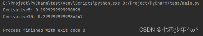
# x=5的导数
x_data = 5
Derivative5 = numerical_diff(function1, x_data)
print('Derivative5:', Derivative5)

# x=10的导数
x_data = 10
Derivative10 = numerical_diff(function1, x_data)
print('Derivative10:', Derivative10)

3).结果展示：

2.偏导数

有多个变量函数的导数称为偏导数。

1).示例：

• 说明：
  ①.公式中有两个变量，所以需要区分对哪个变量求导数，用数学式表示的话，可以写成∂f/∂x0,∂f/∂x1

2).代码实现：

# f(x)=x0^2+x1^2
def numerical_diff(f, x):
    h = 1e-4
    return (f(x + h) - f(x - h)) / (2 * h)


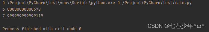
# 当x0=3,x1=4时，关于x0的偏导数∂f/∂x0
def function1(x0):
    return x0 ** 2 + 4.0 ** 2


# 当x0=3,x1=4时，关于x1的偏导数∂f/∂x1
def function2(x1):
    return 3.0 ** 2 + x1 ** 2


# 当x0=3,x1=4时，关于x0的偏导数∂f/∂x0
x = 3.0
y = numerical_diff(function1, x)
print(y)

# 当x0=3,x1=4时，关于x1的偏导数∂f/∂x1
x = 4.0
y = numerical_diff(function2, x)
print(y)

3).结果展示：

3.梯度

在刚才的例子中，我们按变量分别计算x0和x1的偏导数，现在我们希望一起计算x0和x1的偏导数(∂f/∂x0,∂f/∂x1)，像(∂f/∂x0,∂f/∂x1)这样由全部变量的偏导数汇总而成的向量称为梯度。

1).示例：

• 以上述示例为例的代码：

import numpy as np

def function(x):
    return np.sum(x ** 2)


def numerical_gradient(f, x):
    h = 1e-4
    grad = np.zeros_like(x)

    for i in range(x.size):
        # f(x+h)
        fx1 = f(x[i] + h)
        # f(x-h)
        fx2 = f(x[i] - h)

        grad[i] = (fx1 - fx2) / (2 * h)

    return grad


x_data = np.array([3.0, 4.0])
y_data = numerical_gradient(function, x_data)
print(y_data)#output：[6. 8.]

x_data = np.array([0.0, 2.0])
y_data = numerical_gradient(function, x_data)
print(y_data)#output：[0. 4.]

x_data = np.array([3.0, 0.0])
y_data = numerical_gradient(function, x_data)
print(y_data)#output：[6. 0.]

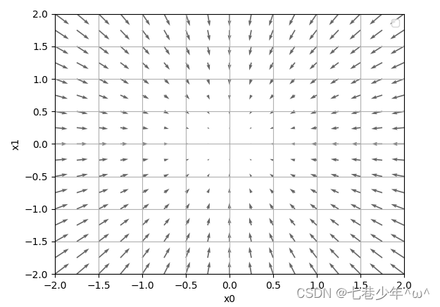
2).图像描述：

• ①.如图所示，f(x0,x1)=x0² +x1²的梯度呈现为有向向量(箭头)，我们发现梯度指向函数f(x)的"最低处"(最小值),就像指南针一样，所有箭头都指向同一点，其次我们发现离“最低处”越远，箭头越大。

  ②.梯度指示的方向是各点处函数值减少最多的方向。

4.梯度法

在梯度法中，函数的取值从当前位置沿着梯度方向前进一定距离，然后在新的位置重新求梯度，在沿着新的梯度方向前进，如何反复，不断沿着梯度方向前进，逐渐减少函数值的过程称为梯度法。

1).梯度法存在的缺陷：

• 梯度表示的是各点处的函数值减小最多的方向，因此无法保证梯度所指向的方向就是函数的最小值或者真正应该前进的方向，可能是局部极小值或者鞍点。[局部极小值：限定在某个范围内的最小值；鞍点：从某个方向上看极大值，从另一个方向上看则是极小值的点]

2).数学式表示梯度：

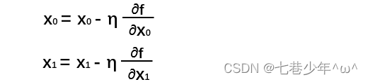
• 参数说明：
  η：学习率

5.学习算法的实现

1).神经网络的学习步骤：

• 前提：
  神经网络存在合适的权重和偏置，调整权重和偏置以便拟合训练数据的过程称为“学习”，神经网络的学习分成下面4个步骤。

• 步骤1 (mini-batch):
  从训练数据中随机选出一部分数据，这部分数据称为mini-batch,我们的目标是减少mini-batch损失函数的值。

• 步骤2 (计算梯度):
  为了减少mini_batch损失函数的值，需要求出各个权重参数的梯度，梯度表示损失函数的值减少最多的方向。

• 步骤3 (更新参数):
  将权重参数沿梯度方向进行微小更新

• 步骤4 (重复)：
  重复步骤1，步骤2，步骤3

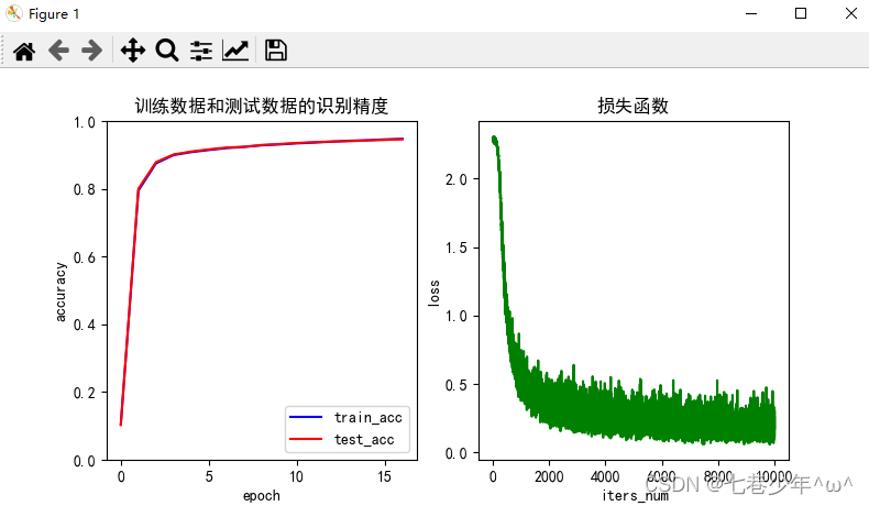
2).示例：(手写数字识别2层神经网络的实现)

import numpy as np
import matplotlib.pyplot as plt
import sys, os

sys.path.append(os.pardir)
from dataset.mnist import load_mnist


# 加载训练数据
def get_data():
    (x_train, t_train), (x_test, t_test) = load_mnist(normalize=True, one_hot_label=True)
    return (x_train, t_train), (x_test, t_test)


# 2层神经网络的类
class TwoLayerNet:
    # 参数初始化
    def __init__(self, input_size, hidden_size, output_size, weight_init_std=0.01):
        self.params = {}
        self.params['W1'] = weight_init_std * np.random.randn(input_size, hidden_size)
        self.params['b1'] = np.zeros(hidden_size)
        self.params['W2'] = weight_init_std * np.random.randn(hidden_size, output_size)
        self.params['b2'] = np.zeros(output_size)

    # 激活函数：sigmoid
    def sigmoid(self, x):
        return 1 / (1 + np.exp(-x))

    # 输出层函数：softmax
    def softmax(self, x):
        if x.ndim == 2:
            x = x.T
            x = x - np.max(x, axis=0)
            y = np.exp(x) / np.sum(np.exp(x), axis=0)
            return y.T

        x = x - np.max(x)  # 溢出对策
        return np.exp(x) / np.sum(np.exp(x))

    def sigmoid_grad(self, x):
        return (1.0 - self.sigmoid(x)) * self.sigmoid(x)

    # 微分函数
    def numerical_gradient(self, f, x):
        h = 1e-4  # 0.0001
        grad = np.zeros_like(x)

        it = np.nditer(x, flags=['multi_index'],
                       op_flags=['readwrite'])  # 多维迭代，遍历数组.为了在遍历数组的同时，实现对数组元素值得修改，必须指定op_flags=['readwrite']模式
        while not it.finished:
            idx = it.multi_index
            tmp_val = x[idx]
            x[idx] = float(tmp_val) + h
            fxh1 = f(x)  # f(x+h)

            x[idx] = tmp_val - h
            fxh2 = f(x)  # f(x-h)
            grad[idx] = (fxh1 - fxh2) / (2 * h)

            x[idx] = tmp_val  # 还原值
            it.iternext()

        return grad

    # 推理函数
    def predict(self, x):
        W1, W2 = self.params['W1'], self.params['W2']
        b1, b2 = self.params['b1'], self.params['b2']

        # 第一层
        a1 = np.dot(x, W1) + b1
        z1 = self.sigmoid(a1)

        # 第二层
        a2 = np.dot(z1, W2) + b2
        y = self.softmax(a2)

        return y

    # 交叉熵误差
    def cross_entropy_error(self, y, t):
        if y.ndim == 1:
            t = t.reshape(1, t.size)
            y = y.reshape(1, y.size)

        # 监督数据是one-hot-vector的情况下，转换为正确解标签的索引
        if t.size == y.size:
            t = t.argmax(axis=1)

        batch_size = y.shape[0]
        return -np.sum(np.log(y[np.arange(batch_size), t] + 1e-7)) / batch_size

    # 损失函数
    def loss(self, x, t):
        y = self.predict(x)
        loss = self.cross_entropy_error(y, t)
        return loss

    # 识别精度
    def Accuracy(self, x, t):
        y = self.predict(x)
        y = np.argmax(y, axis=1)
        t = np.argmax(t, axis=1)

        accuracy = np.sum(y == t) / float(x.shape[0])

        return accuracy

    # 梯度法
    def numerical_gradient(self, x, t):
        loss_W = lambda W: self.loss(x, t)

        grads = {}
        grads['W1'] = self.numerical_gradient(loss_W, self.params['W1'])
        grads['b1'] = self.numerical_gradient(loss_W, self.params['b1'])
        grads['W2'] = self.numerical_gradient(loss_W, self.params['W2'])
        grads['b2'] = self.numerical_gradient(loss_W, self.params['b2'])

        return grads

    def gradient(self, x, t):
        W1, W2 = self.params['W1'], self.params['W2']
        b1, b2 = self.params['b1'], self.params['b2']
        grads = {}

        batch_num = x.shape[0]

        # forward
        a1 = np.dot(x, W1) + b1
        z1 = self.sigmoid(a1)
        a2 = np.dot(z1, W2) + b2
        y = self.softmax(a2)

        # backward
        dy = (y - t) / batch_num
        grads['W2'] = np.dot(z1.T, dy)
        grads['b2'] = np.sum(dy, axis=0)

        da1 = np.dot(dy, W2.T)
        dz1 = self.sigmoid_grad(a1) * da1
        grads['W1'] = np.dot(x.T, dz1)
        grads['b1'] = np.sum(dz1, axis=0)

        return grads


# 加载训练数据
(x_train, t_train), (x_test, t_test) = get_data()

train_loss_list = []
train_acc_list = []
test_acc_list = []

# 超参数
iters_num = 10000
lr = 0.1
batch_size = 100
train_size = x_train.shape[0]

# 平均每个epoch的重复次数
iter_per_epoch = max(train_size / batch_size, 1)

network = TwoLayerNet(input_size=784, hidden_size=50, output_size=10)

for i in range(iters_num):

    # 获取mini-batch
    batch_mask = np.random.choice(train_size, batch_size)
    x_batch = x_train[batch_mask]
    t_batch = t_train[batch_mask]

    # 计算梯度
    # grad = network.numerical_gradient(x_batch, t_batch)
    grad = network.gradient(x_batch, t_batch)

    # 参数更新
    for key in ('W1', 'b1', 'W2', 'b2'):
        network.params[key] -= lr * grad[key]

    # 记录学习过程
    loss = network.loss(x_batch, t_batch)
    train_loss_list.append(loss)

    # 计算每个epoch的识别精度
    if i % iter_per_epoch == 0:
        train_acc = network.Accuracy(x_train, t_train)
        test_acc = network.Accuracy(x_test, t_test)
        train_acc_list.append(train_acc)
        test_acc_list.append(test_acc)
        print("train acc,test acc|" + str(train_acc) + ',' + str(test_acc))

# 绘制识别精度图像
plt.rcParams['font.sans-serif'] = ['SimHei']  # 解决中文乱码
plt.rcParams['axes.unicode_minus'] = False  # 解决负号不显示的问题

plt.figure(figsize=(8, 4))
plt.subplot(1, 2, 1)
x_data = np.arange(0, len(train_acc_list))
plt.plot(x_data, train_acc_list, 'b')
plt.plot(x_data, test_acc_list, 'r')
plt.xlabel('epoch')
plt.ylabel('accuracy')
plt.ylim(0.0, 1.0)
plt.title('训练数据和测试数据的识别精度')
plt.legend(['train_acc', 'test_acc'])

plt.subplot(1, 2, 2)
x_data = np.arange(0, len(train_loss_list))
plt.plot(x_data, train_loss_list, 'g')
plt.xlabel('iters_num')
plt.ylabel('loss')
plt.title('损失函数')
plt.show()

3).结果展示：