多元数据的直观表示及R使用

Author:龙箬
Data Science and Big Data Technology
Change the world with data!
优快云@weixin_43975035
上帝已死，哲学永生

多元数据的直观表示及R使用

均值条图及R使用

> X=read.table("clipboard",header=T)
> X

运行结果如下：

          食品    衣着   设备    医疗    交通    教育    居住   杂项
北京   4934.05 1512.88 981.13 1294.07 2328.51 2383.96 1246.19 649.66
天津   4249.31 1024.15 760.56 1163.98 1309.94 1639.83 1417.45 463.64
河北   2789.85  975.94 546.75  833.51 1010.51  895.06  917.19 266.16
山西   2600.37 1064.61 477.74  640.22 1027.99 1054.05  991.77 245.07
内蒙古 2824.89 1396.86 561.71  719.13 1123.82 1245.09  941.79 468.17
辽宁   3560.21 1017.65 439.28  879.08 1033.36 1052.94 1047.04 400.16
吉林   2842.68 1127.09 407.35  854.80  873.88  997.75 1062.46 394.29
黑龙江 2633.18 1021.45 355.67  729.55  746.03  938.21  784.51 310.67
上海   6125.45 1330.05 959.49  857.11 3153.72 2653.67 1412.10 763.80
江苏   3928.71  990.03 707.31  689.37 1303.02 1699.26 1020.09 377.37
浙江   4892.58 1406.20 666.02  859.06 2473.40 2158.32 1168.08 467.52
安徽   3384.38  906.47 465.68  554.44  891.38 1169.99  850.24 309.30
福建   4296.22  940.72 645.40  502.41 1606.90 1426.34 1261.18 375.98
江西   3192.61  915.09 587.40  385.91  732.97  973.38  728.76 294.60
山东   3180.64 1238.34 661.03  708.58 1333.63 1191.18 1027.58 325.64
河南   2707.44 1053.13 549.14  626.55  858.33  936.55  795.39 300.19
湖北   3455.98 1046.62 550.16  525.32  903.02 1120.29  856.97 242.82
湖南   3243.88 1017.59 603.18  668.53  986.89 1285.24  869.59 315.82
广东   5056.68  814.57 853.18  752.52 2966.08 1994.86 1444.91 454.09
广西   3398.09  656.69 491.03  542.07  932.87 1050.04  803.04 277.43
海南   3546.67  452.85 519.99  503.78 1401.89  837.83  819.02 210.85
重庆   3674.28 1171.15 706.77  749.51 1118.79 1237.35  968.45 264.01
四川   3580.14  949.74 562.02  511.78 1074.91 1031.81  690.27 291.32
贵州   3122.46  910.30 463.56  354.52  895.04 1035.96  718.65 258.21
云南   3562.33  859.65 280.62  631.70 1034.71  705.51  673.07 174.23
西藏   3836.51  880.10 271.29  272.81  866.33  441.02  628.35 335.66
陕西   3063.69  910.29 513.08  678.38  866.76 1230.74  831.27 332.84
甘肃   2824.42  939.89 505.16  564.25  861.47 1058.66  768.28 353.65
青海   2803.45  898.54 484.71  613.24  785.27  953.87  641.93 331.38
宁夏   2760.74  994.47 480.84  645.98  859.04  863.36  910.68 302.17
新疆   2760.69 1183.69 475.23  598.78  890.30  896.79  736.99 331.80

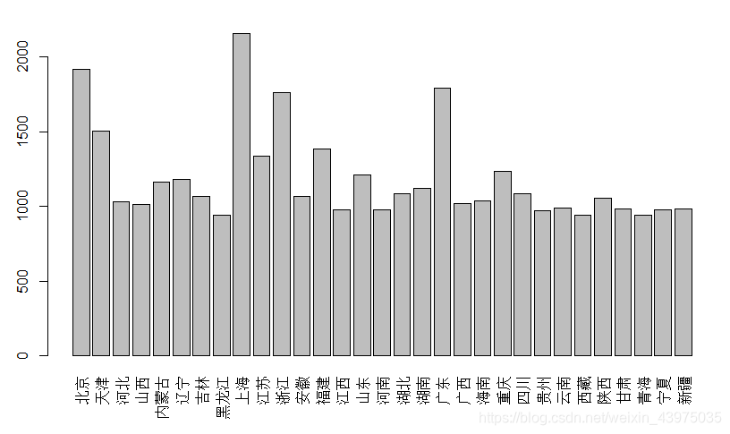
barplot(apply(X,1,mean),las=3) # 按行作均值条形图 

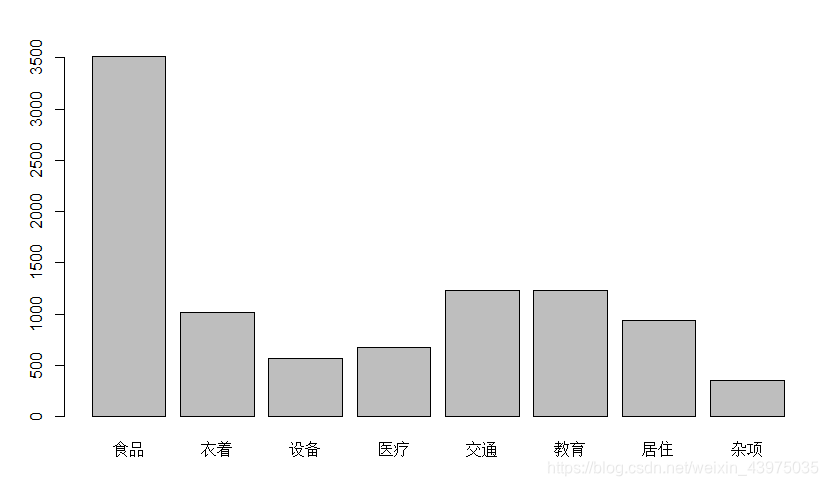
> barplot(apply(X,2,mean)) #按列作均值条形图

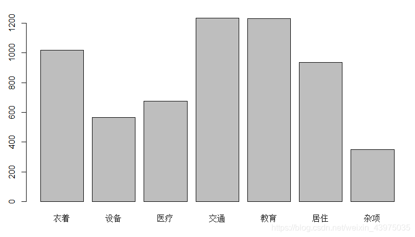
> barplot(apply(X[,2:8],2,mean)) # 去掉第一后的数据按列作均值条形图

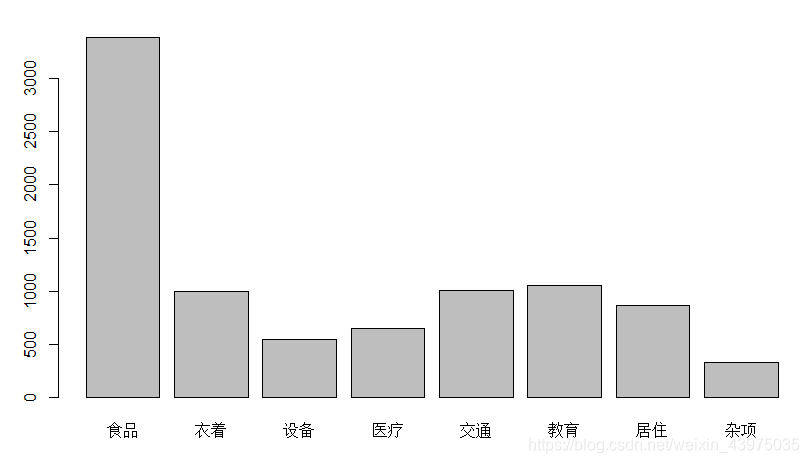
> barplot(apply(X,2,median)) #按列作中位数条形图

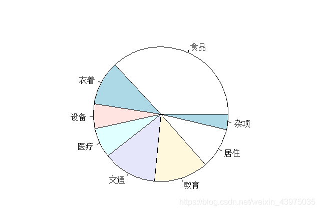
> pie(apply(X,2,mean)) #按列作均值饼图

箱尾图及R使用

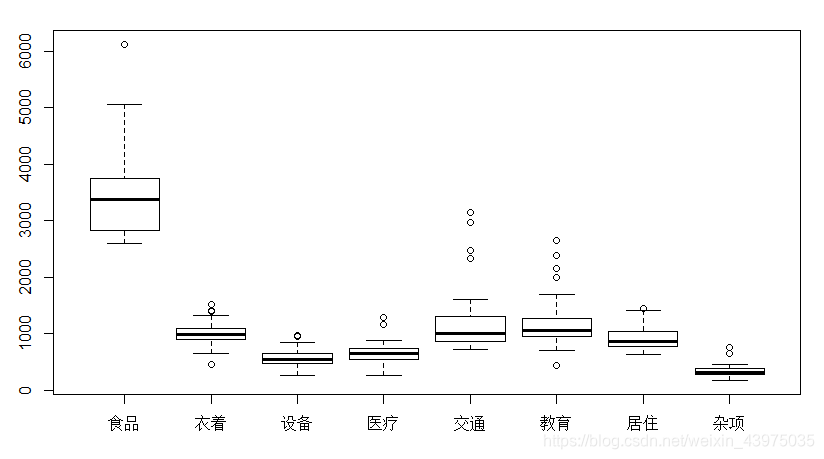
boxplot(X) #按列做箱尾图

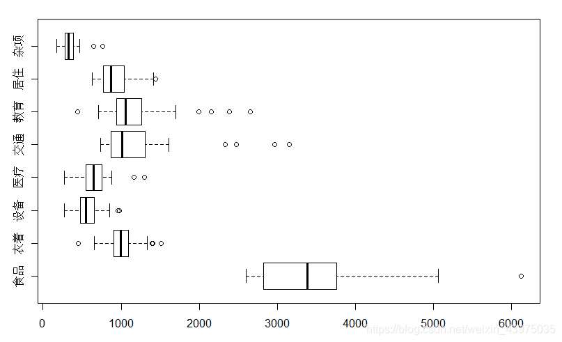
> boxplot(X,horizontal = T) #箱尾图中图形按水平放置

星相图及R使用

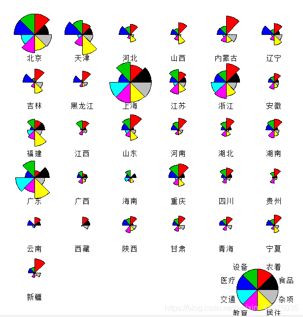
> stars(X,full=T,key.loc = c(13,1.5))# 具有图例的360度星象图

> stars(X,full=F,key.loc = c(13,1.5))# 具有图例的180度星象图

> stars(X,full=T,draw.segments=T,key.loc = c(13,1.5)) #具有图例的360度彩色星象图

> stars(X,full=F,draw.segments=T,key.loc = c(13,1.5)) #具有图例的180度彩色星象图

脸谱图及R使用

加载aplpack包之前应先下载安装

> library(aplpack) #加载aplpack包
> faces(X,ncol.plot=7)

运行结果如下：

effect of variables:
 modified item       Var   
 "height of face   " "食品"
 "width of face    " "衣着"
 "structure of face" "设备"
 "height of mouth  " "医疗"
 "width of mouth   " "交通"
 "smiling          " "教育"
 "height of eyes   " "居住"
 "width of eyes    " "杂项"
 "height of hair   " "食品"
 "width of hair   "  "衣着"
 "style of hair   "  "设备"
 "height of nose  "  "医疗"
 "width of nose   "  "交通"
 "width of ear    "  "教育"
 "height of ear   "  "居住"

> faces(X[,2:8],ncol.plot = 7) #去掉第一个变量按每行7个作脸谱图

运行结果如下：

effect of variables:
 modified item       Var   
 "height of face   " "衣着"
 "width of face    " "设备"
 "structure of face" "医疗"
 "height of mouth  " "交通"
 "width of mouth   " "教育"
 "smiling          " "居住"
 "height of eyes   " "杂项"
 "width of eyes    " "衣着"
 "height of hair   " "设备"
 "width of hair   "  "医疗"
 "style of hair   "  "交通"
 "height of nose  "  "教育"
 "width of nose   "  "居住"
 "width of ear    "  "杂项"
 "height of ear   "  "衣着"

> faces(X[c(1,9,19,20,22,28,31),]) #选择第1,9,19,20,22,28,31个观测的多元数据作脸谱图

运行结果如下：

effect of variables:
 modified item       Var   
 "height of face   " "食品"
 "width of face    " "衣着"
 "structure of face" "设备"
 "height of mouth  " "医疗"
 "width of mouth   " "交通"
 "smiling          " "教育"
 "height of eyes   " "居住"
 "width of eyes    " "杂项"
 "height of hair   " "食品"
 "width of hair   "  "衣着"
 "style of hair   "  "设备"
 "height of nose  "  "医疗"
 "width of nose   "  "交通"
 "width of ear    "  "教育"
 "height of ear   "  "居住"

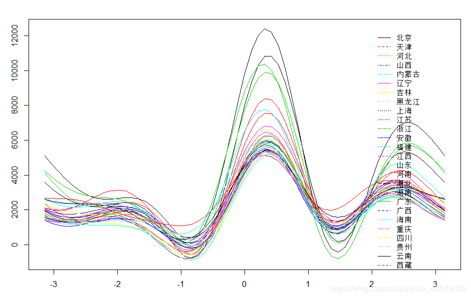
调和曲线图及R使用

由于R语言4.0版本好像不支持mvstats的使用，因此本人使用R语言3.6.3版本进行下载并安装mvstats库，需要mvstats的小伙伴请联系博客作者（联系方式见文末）

> .libPaths() #用来查看当前的正在使用的库是哪个
[1] "D:/R/R-3.6.3/library"

> library(mvstats)
> plot.andrews(X)

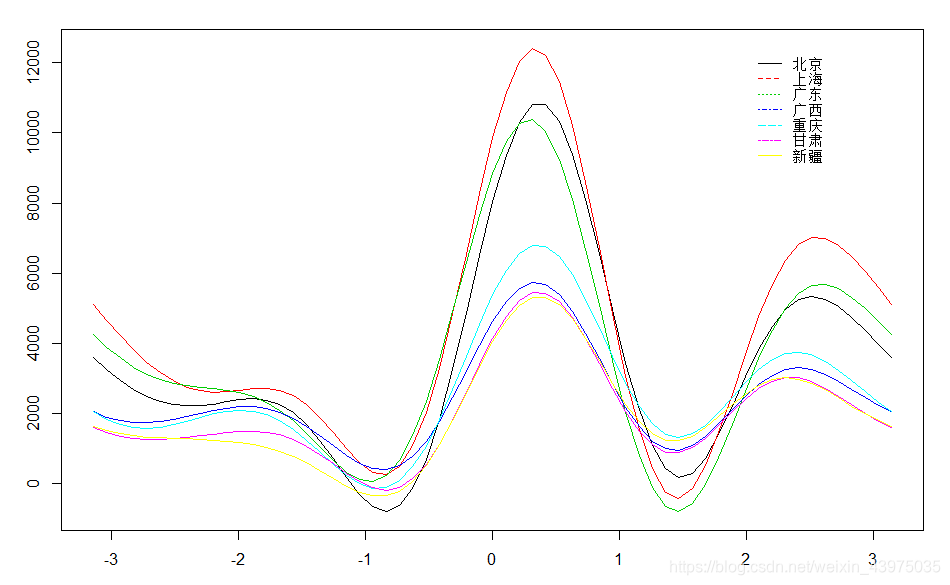
> plot.andrews(X[c(1,9,19,20,22,28,31),])# #选择第1,9,19,20,22,28,31个观测的调和曲线图

参考致谢：
王斌会.多元统计分析及R语言建模（第四版）

如有侵权，请联系侵删
需要本实验源数据及代码的小伙伴请联系QQ:2225872659