深度学习TensorFlow入门

最新推荐文章于 2020-10-18 17:25:43 发布

Jason Mraz

最新推荐文章于 2020-10-18 17:25:43 发布

阅读量442

点赞数 1

分类专栏：深度学习文章标签： python 深度学习机器学习 TensorFlow 神经网络

本文链接：https://blog.youkuaiyun.com/weixin_43937114/article/details/85133649

版权

深度学习专栏收录该内容

0 篇文章

订阅专栏

这篇博客介绍了TensorFlow的基础知识，包括如何安装TensorFlow，展示了简单的使用方法，并通过一个线性回归的例子详细解释了如何使用TensorFlow实现机器学习模型。适合初学者入门。

摘要生成于 C知道，由 DeepSeek-R1 满血版支持，前往体验 >

TensorFlow基础

TensorFlow是一个基于数据流编程（dataflow programming）的符号数学系统，被广泛应用于各类机器学习（machine learning）算法的编程实现，其前身是谷歌的神经网络算法库DistBelief。

安装

这里使用的是Anaconda安装，打开黑窗口(Anaconda Prompt)，输入命令：

pip install tensorflow

在这里插入图片描述
或者在图形界面环境，Not installed 搜索 tensorflow,点击安装即可。

简单用法

import tensorflow as tf

# Simple hello world using TensorFlow

# Create a Constant op
# The op is added as a node to the default graph.
#
# The value returned by the constructor represents the output
# of the Constant op.

#定义一个常量
hello = tf.constant("Hello, Tensorflow")

#Start tf Session
sess = tf.Session()

#run graph  执行流图
print(sess.run(hello))

在这里插入图片描述

#session close
sess.close()

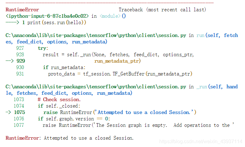
操作关闭后不能继续执行使用，提示报错

print(sess.run(hello))

在这里插入图片描述

使用TensorFlow实现线性回归

Linear Regression Example

导包

import numpy as np
import tensorflow as tf
import matplotlib.pyplot as plt
%matplotlib inline
rng = np.random

定义训练次数learning_epochs，卷曲神经的学习率learning_rate
显示打印数据的步幅display_step

learning_epochs = 1000
learning_rate = 0.01
display_step = 50

生成训练数据

train_X = np.linspace(0,10,num = 20)+rng.randn(20)
train_X

在这里插入图片描述

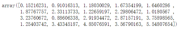
train_Y = np.linspace(1,4,num = 20)+rng.randn(20)
train_Y

在这里插入图片描述

n_samples = train_Y.shape[0]
n_samples

在这里插入图片描述

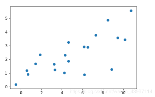
plt.scatter(train_X,train_Y)

在这里插入图片描述

定义TensorFlow参数：X，Y，W，b

X = tf.placeholder("float")
Y = tf.placeholder("float")

#Variable里面定义了斜率和截距
#weight  权重
#bias    偏差，相当于截距
W = tf.Variable(rng.randn(), name = "weight")
b = tf.Variable(rng.randn(), name = "bias")

创建线性模型

y_pred = tf.add(tf.multiply(W,X), b)
#y = w*x + b

创建TensorFlow均方误差cost
以及梯度下降优化器optimizer

例：reduce_sum用法

a = tf.constant([1,2,3])
sess = tf.Session()
sess.run(tf.reduce_sum(a))

在这里插入图片描述

#损失，误差
#均方误差，严格的按照最小二乘法
cost = tf.reduce_sum(tf.pow((y_pred - Y),2))/n_samples

#如何把cost变为最小？  梯度下降算法
#就是一个操作
optimizer = tf.train.GradientDescentOptimizer(learning_rate).minimize(cost)

TensorFlow进行初始化

init = tf.global_variables_initializer()
#对tensorflow  进行初始化的

#开始训练
with tf.Session() as sess:
    #开始初始化
    sess.run(init)
    #训练所有数据,1000次循环
    for epoch in range(learning_epochs):
        #执行20次
        for (x,y) in zip(train_X,train_Y):
            #每次执行梯度下降算法
            sess.run(optimizer, feed_dict= {X:x, Y:y})
        #每执行50次然后打印一下损失值
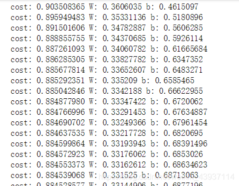
        if (epoch+1)%display_step == 0:
            #cost均方误差
            c = sess.run(cost, feed_dict={X:train_X, Y:train_Y})
            print("cost:","{:.9f}".format(c), "W:",sess.run(W), "b:",sess.run(b))
            
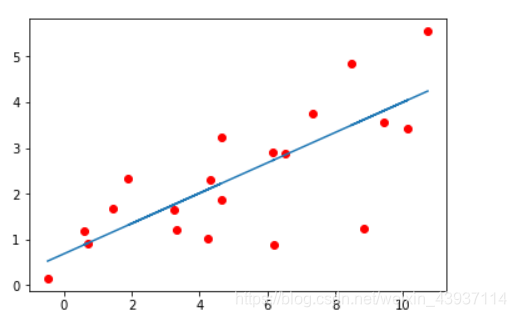
    #数据可视化
    plt.plot(train_X, train_Y, "ro")
    plt.plot(train_X, sess.run(W)*train_X+sess.run(b))

在这里插入图片描述