T2 TensorFlow入门实战——彩色图片分类

• 🍨 本文為🔗365天深度學習訓練營 中的學習紀錄博客
• 🍖 原作者：K同学啊 | 接輔導、項目定制

一、前期准备

1. 导入数据

# Import the required libraries
import tensorflow as tf
from tensorflow.keras import datasets, layers, models
import matplotlib.pyplot as plt
import numpy as np

# 导入cifar10数据，依次分别为训练集图片、训练集标签、测试集图片、测试集标签
(train_images, train_labels), (test_images, test_labels) = datasets.cifar10.load_data()

2. 归一化

# Normalize pixel values to be between 0 and 1
train_images, test_images = train_images / 255.0, test_images / 255.0
# Check the shape of the data
print("Training data shape:", train_images.shape)
print("Training labels shape:", train_labels.shape)
print("Testing data shape:", test_images.shape)
print("Testing labels shape:", test_labels.shape)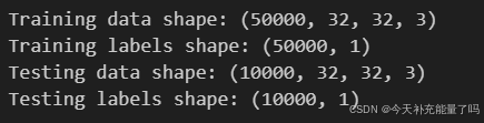

3. 可视化

展示数据集前20张图片

# Plot the first 20 images
class_names = ['airplane', 'automobile', 'bird', 'cat', 'deer','dog', 'frog', 'horse', 'ship', 'truck']

# 进行图像大小为20宽、10长的绘图(单位为英寸inch)
plt.figure(figsize=(20,10))
# 遍历MNIST数据集下标数值0~49
for i in range(20):
    # 将整个figure分成5行10列，绘制第i+1个子图。
    plt.subplot(5,10,i+1)
    # 设置不显示x轴刻度
    plt.xticks([])
    # 设置不显示y轴刻度
    plt.yticks([])
    # 设置不显示子图网格线
    plt.grid(False)
    # 图像展示，cmap为颜色图谱，"plt.cm.binary"为matplotlib.cm中的色表
    plt.imshow(train_images[i], cmap=plt.cm.binary)
    # 设置x轴标签显示为图片对应的数字
    plt.xlabel(class_names[train_labels[i][0]])
# 显示图片
plt.show()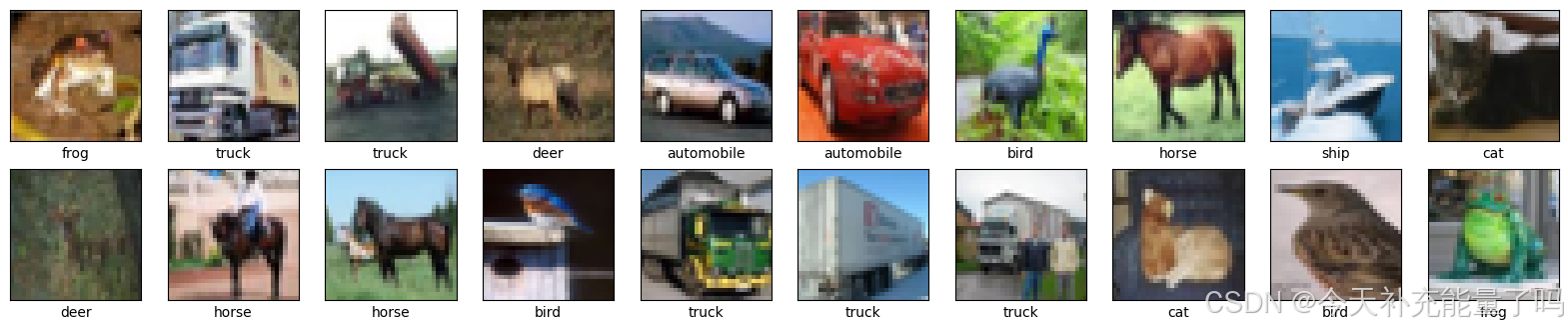

二、训练模型 

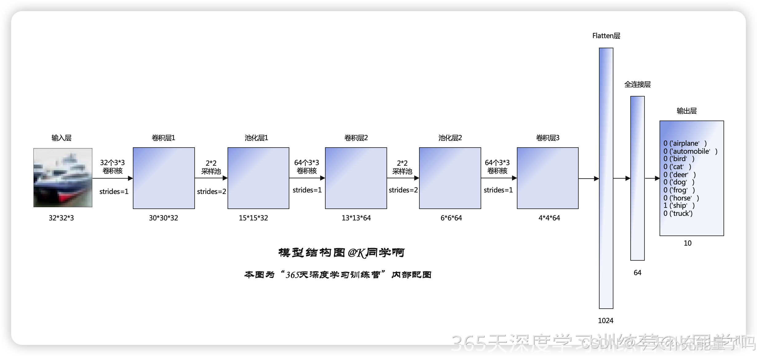
1. 构建CNN网络模型

⭐池化层

池化层对提取到的特征信息进行降维，一方面使特征图变小，简化网络计算复杂度；另一方面进行特征压缩，提取主要特征，增加平移不变性，减少过拟合风险。但其实池化更多程度上是一种计算性能的一个妥协，强硬地压缩特征的同时也损失了一部分信息，所以现在的网络比较少用池化层或者使用优化后的如SoftPool。

池化层包括最大池化层（MaxPooling）和平均池化层（AveragePooling），均值池化对背景保留更好，最大池化对纹理提取更好）。同卷积计算，池化层计算窗口内的平均值或者最大值。

# Define the model architecture
# 创建并设置卷积神经网络
# 卷积层：通过卷积操作对输入图像进行降维和特征抽取
# 池化层：是一种非线性形式的下采样。主要用于特征降维，压缩数据和参数的数量，减小过拟合，同时提高模型的鲁棒性。
# 全连接层：在经过几个卷积和池化层之后，神经网络中的高级推理通过全连接层来完成。
model = models.Sequential([
    layers.Conv2D(32, (3, 3), activation='relu', input_shape=(32, 32, 3)), #卷积层1，卷积核3*3
    layers.MaxPooling2D((2, 2)),                   #池化层1，2*2采样
    layers.Conv2D(64, (3, 3), activation='relu'),  #卷积层2，卷积核3*3
    layers.MaxPooling2D((2, 2)),                   #池化层2，2*2采样
    layers.Conv2D(64, (3, 3), activation='relu'),  #卷积层3，卷积核3*3
    
    layers.Flatten(),                      #Flatten层，连接卷积层与全连接层
    layers.Dense(64, activation='relu'),   #全连接层，特征进一步提取
    layers.Dense(10)                       #输出层，输出预期结果
])

model.summary()  # 打印网络结构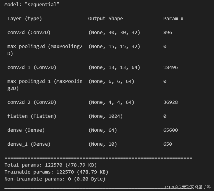

2. 编译模型

"""
这里设置优化器、损失函数以及metrics
"""
# model.compile()方法用于在配置训练方法时，告知训练时用的优化器、损失函数和准确率评测标准
model.compile(
	# 设置优化器为Adam优化器
    optimizer='adam',
	# 设置损失函数为交叉熵损失函数（tf.keras.losses.SparseCategoricalCrossentropy()）
    # from_logits为True时，会将y_pred转化为概率（用softmax），否则不进行转换，通常情况下用True结果更稳定
    loss=tf.keras.losses.SparseCategoricalCrossentropy(from_logits=True),
    # 设置性能指标列表，将在模型训练时监控列表中的指标
    metrics=['accuracy'])

3. 训练模型

"""
这里设置输入训练数据集（图片及标签）、验证数据集（图片及标签）以及迭代次数epochs
关于model.fit()函数的具体介绍可参考我的博客：
https://blog.youkuaiyun.com/qq_38251616/article/details/122321757
"""
history = model.fit(
    # 输入训练集图片
	train_images, 
	# 输入训练集标签
	train_labels, 
	# 设置10个epoch，每一个epoch都将会把所有的数据输入模型完成一次训练。
	epochs=10, 
	# 设置验证集
    validation_data=(test_images, test_labels))

Epoch 1/10
1563/1563 [==============================] - 55s 32ms/step - loss: 1.5203 - accuracy: 0.4440 - val_loss: 1.2369 - val_accuracy: 0.5617
Epoch 2/10
1563/1563 [==============================] - 64s 41ms/step - loss: 1.1512 - accuracy: 0.5936 - val_loss: 1.0745 - val_accuracy: 0.6187
Epoch 3/10
1563/1563 [==============================] - 55s 35ms/step - loss: 0.9915 - accuracy: 0.6511 - val_loss: 0.9783 - val_accuracy: 0.6594
Epoch 4/10
1563/1563 [==============================] - 58s 37ms/step - loss: 0.8915 - accuracy: 0.6851 - val_loss: 0.9429 - val_accuracy: 0.6726
Epoch 5/10
1563/1563 [==============================] - 67s 43ms/step - loss: 0.8243 - accuracy: 0.7114 - val_loss: 0.9159 - val_accuracy: 0.6821
Epoch 6/10
1563/1563 [==============================] - 47s 30ms/step - loss: 0.7612 - accuracy: 0.7333 - val_loss: 0.8799 - val_accuracy: 0.6933
Epoch 7/10
1563/1563 [==============================] - 50s 32ms/step - loss: 0.7116 - accuracy: 0.7476 - val_loss: 0.8523 - val_accuracy: 0.7048
Epoch 8/10
1563/1563 [==============================] - 71s 45ms/step - loss: 0.6727 - accuracy: 0.7632 - val_loss: 0.9358 - val_accuracy: 0.6889
Epoch 9/10
1563/1563 [==============================] - 48s 31ms/step - loss: 0.6334 - accuracy: 0.7762 - val_loss: 0.9098 - val_accuracy: 0.6977
Epoch 10/10
1563/1563 [==============================] - 51s 32ms/step - loss: 0.5931 - accuracy: 0.7912 - val_loss: 0.8912 - val_accuracy: 0.7066

三、模型预测 

通过模型进行预测得到的是每一个类别的概率，数字越大该图片为该类别的可能性越大

plt.imshow(test_images[1])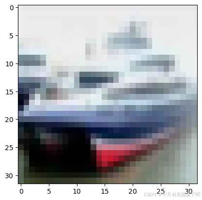

# 输出测试集图片的预测结果
pre = model.predict(test_images) # 对所有测试图片进行预测
print(class_names[np.argmax(pre[1])]) # 输出第一张图片的预测结果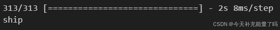

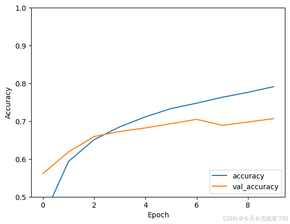
四、模型评估

# Evaluate the model 
plt.plot(history.history['accuracy'], label='accuracy')
plt.plot(history.history['val_accuracy'], label = 'val_accuracy')
plt.xlabel('Epoch')
plt.ylabel('Accuracy')
plt.ylim([0.5, 1])
plt.legend(loc='lower right')
plt.show()

test_loss, test_acc = model.evaluate(test_images,  test_labels, verbose=2)

print(test_acc)