


- 🍨 本文為🔗365天深度學習訓練營 中的學習紀錄博客
- 🍖 原作者:K同学啊 | 接輔導、項目定制
一、前期准备
1. 设置device
# import the necessary libraries
import torch
import torch.nn as nn
import torchvision.transforms as transforms
from torchvision import transforms, datasets
from torchvision.models import vgg16
import matplotlib.pyplot as plt
import PIL,pathlib
from PIL import Image
#隐藏警告
import warnings
import copy
import torchsummary as summary
warnings.filterwarnings("ignore")               #忽略警告信息
plt.rcParams['font.sans-serif']    = ['SimHei'] # 用来正常显示中文标签
plt.rcParams['axes.unicode_minus'] = False      # 用来正常显示负号
plt.rcParams['figure.dpi']         = 100        #分辨率

# 设置硬件设备,如果有GPU则使用,没有则使用cpu
device = torch.device("cuda" if torch.cuda.is_available() else "cpu")
device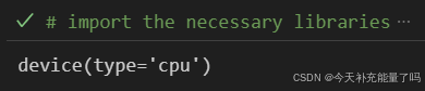
2. 导入数据
# load the data
data_dir = './data/PotatoPlants/'
data_dir = pathlib.Path(data_dir)

data_paths = list(data_dir.glob('*'))
classeNames = [str(path).split("\\")[2] for path in data_paths]
classeNames![]()
# 关于transforms.Compose的更多介绍可以参考:https://blog.youkuaiyun.com/qq_38251616/article/details/124878863
train_transforms = transforms.Compose([
    transforms.Resize([224, 224]),  # 将输入图片resize成统一尺寸
    # transforms.RandomHorizontalFlip(), # 随机水平翻转
    transforms.ToTensor(),          # 将PIL Image或numpy.ndarray转换为tensor,并归一化到[0,1]之间
    transforms.Normalize(           # 标准化处理-->转换为标准正太分布(高斯分布),使模型更容易收敛
        mean=[0.485, 0.456, 0.406],
        std=[0.229, 0.224, 0.225])  # 其中 mean=[0.485,0.456,0.406]与std=[0.229,0.224,0.225] 从数据集中随机抽样计算得到的。
])

test_transform = transforms.Compose([
    transforms.Resize([224, 224]),  # 将输入图片resize成统一尺寸
    transforms.ToTensor(),          # 将PIL Image或numpy.ndarray转换为tensor,并归一化到[0,1]之间
    transforms.Normalize(           # 标准化处理-->转换为标准正太分布(高斯分布),使模型更容易收敛
        mean=[0.485, 0.456, 0.406],
        std=[0.229, 0.224, 0.225])  # 其中 mean=[0.485,0.456,0.406]与std=[0.229,0.224,0.225] 从数据集中随机抽样计算得到的。
])

total_data = datasets.ImageFolder("./data/PotatoPlants/", transform=train_transforms)
total_data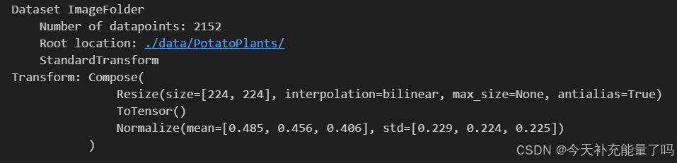
total_data.class_to_idx![]()
3. 划分数据集
# Split the data into training and test sets
train_size = int(0.8 * len(total_data))
test_size  = len(total_data) - train_size
train_dataset, test_dataset = torch.utils.data.random_split(total_data, [train_size, test_size])
train_dataset, test_dataset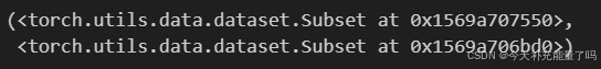
batch_size = 32

train_dl = torch.utils.data.DataLoader(train_dataset,
                                           batch_size=batch_size,
                                           shuffle=True,
                                           num_workers=0)
test_dl = torch.utils.data.DataLoader(test_dataset,
                                          batch_size=batch_size,
                                          shuffle=True,
                                          num_workers=0)

for X, y in test_dl:
    print("Shape of X [N, C, H, W]: ", X.shape)
    print("Shape of y: ", y.shape, y.dtype)
    break
二、手动搭建VGG-16模型
1. 搭建模型
# Define the model
class vgg16(nn.Module):
    def __init__(self):
        super(vgg16, self).__init__()
        # 卷积块1
        self.block1 = nn.Sequential(
            nn.Conv2d(3, 64, kernel_size=(3, 3), stride=(1, 1), padding=(1, 1)),
            nn.ReLU(),
            nn.Conv2d(64, 64, kernel_size=(3, 3), stride=(1, 1), padding=(1, 1)),
            nn.ReLU(),
            nn.MaxPool2d(kernel_size=(2, 2), stride=(2, 2))
        )
        # 卷积块2
        self.block2 = nn.Sequential(
            nn.Conv2d(64, 128, kernel_size=(3, 3), stride=(1, 1), padding=(1, 1)),
            nn.ReLU(),
            nn.Conv2d(128, 128, kernel_size=(3, 3), stride=(1, 1), padding=(1, 1)),
            nn.ReLU(),
            nn.MaxPool2d(kernel_size=(2, 2), stride=(2, 2))
        )
        # 卷积块3
        self.block3 = nn.Sequential(
            nn.Conv2d(128, 256, kernel_size=(3, 3), stride=(1, 1), padding=(1, 1)),
            nn.ReLU(),
            nn.Conv2d(256, 256, kernel_size=(3, 3), stride=(1, 1), padding=(1, 1)),
            nn.ReLU(),
            nn.Conv2d(256, 256, kernel_size=(3, 3), stride=(1, 1), padding=(1, 1)),
            nn.ReLU(),
            nn.MaxPool2d(kernel_size=(2, 2), stride=(2, 2))
        )
        # 卷积块4
        self.block4 = nn.Sequential(
            nn.Conv2d(256, 512, kernel_size=(3, 3), stride=(1, 1), padding=(1, 1)),
            nn.ReLU(),
            nn.Conv2d(512, 512, kernel_size=(3, 3), stride=(1, 1), padding=(1, 1)),
            nn.ReLU(),
            nn.Conv2d(512, 512, kernel_size=(3, 3), stride=(1, 1), padding=(1, 1)),
            nn.ReLU(),
            nn.MaxPool2d(kernel_size=(2, 2), stride=(2, 2))
        )
        # 卷积块5
        self.block5 = nn.Sequential(
            nn.Conv2d(512, 512, kernel_size=(3, 3), stride=(1, 1), padding=(1, 1)),
            nn.ReLU(),
            nn.Conv2d(512, 512, kernel_size=(3, 3), stride=(1, 1), padding=(1, 1)),
            nn.ReLU(),
            nn.Conv2d(512, 512, kernel_size=(3, 3), stride=(1, 1), padding=(1, 1)),
            nn.ReLU(),
            nn.MaxPool2d(kernel_size=(2, 2), stride=(2, 2))
        )


        # 全连接网络层,用于分类
        self.classifier = nn.Sequential(
            nn.Linear(in_features=512*7*7, out_features=4096),
            nn.ReLU(),
            nn.Linear(in_features=4096, out_features=4096),
            nn.ReLU(),
            nn.Linear(in_features=4096, out_features=3)
        )

    def forward(self, x):

        x = self.block1(x)
        x = self.block2(x)
        x = self.block3(x)
        x = self.block4(x)
        x = self.block5(x)
        x = torch.flatten(x, start_dim=1)
        x = self.classifier(x)

        return x

device = "cuda" if torch.cuda.is_available() else "cpu"
print("Using {} device".format(device))


model = vgg16().to(device)
model
2. 查看模型详情
如果没安装torchsummary需要先使用pip进行安装
# Check the model summary
summary.summary(model, (3, 224, 224))
----------------------------------------------------------------
Layer (type) Output Shape Param #
================================================================
Conv2d-1 [-1, 64, 224, 224] 1,792
ReLU-2 [-1, 64, 224, 224] 0
Conv2d-3 [-1, 64, 224, 224] 36,928
ReLU-4 [-1, 64, 224, 224] 0
MaxPool2d-5 [-1, 64, 112, 112] 0
Conv2d-6 [-1, 128, 112, 112] 73,856
ReLU-7 [-1, 128, 112, 112] 0
Conv2d-8 [-1, 128, 112, 112] 147,584
ReLU-9 [-1, 128, 112, 112] 0
MaxPool2d-10 [-1, 128, 56, 56] 0
Conv2d-11 [-1, 256, 56, 56] 295,168
ReLU-12 [-1, 256, 56, 56] 0
Conv2d-13 [-1, 256, 56, 56] 590,080
ReLU-14 [-1, 256, 56, 56] 0
Conv2d-15 [-1, 256, 56, 56] 590,080
ReLU-16 [-1, 256, 56, 56] 0
MaxPool2d-17 [-1, 256, 28, 28] 0
Conv2d-18 [-1, 512, 28, 28] 1,180,160
ReLU-19 [-1, 512, 28, 28] 0
Conv2d-20 [-1, 512, 28, 28] 2,359,808
ReLU-21 [-1, 512, 28, 28] 0
Conv2d-22 [-1, 512, 28, 28] 2,359,808
ReLU-23 [-1, 512, 28, 28] 0
MaxPool2d-24 [-1, 512, 14, 14] 0
Conv2d-25 [-1, 512, 14, 14] 2,359,808
ReLU-26 [-1, 512, 14, 14] 0
Conv2d-27 [-1, 512, 14, 14] 2,359,808
ReLU-28 [-1, 512, 14, 14] 0
Conv2d-29 [-1, 512, 14, 14] 2,359,808
ReLU-30 [-1, 512, 14, 14] 0
MaxPool2d-31 [-1, 512, 7, 7] 0
Linear-32 [-1, 4096] 102,764,544
ReLU-33 [-1, 4096] 0
Linear-34 [-1, 4096] 16,781,312
ReLU-35 [-1, 4096] 0
Linear-36 [-1, 3] 12,291
================================================================
Total params: 134,272,835
Trainable params: 134,272,835
Non-trainable params: 0
----------------------------------------------------------------
Input size (MB): 0.57
Forward/backward pass size (MB): 218.52
Params size (MB): 512.21
Estimated Total Size (MB): 731.30
----------------------------------------------------------------三、 训练模型
1. 编写训练函数
# Define the training function
def train(dataloader, model, loss_fn, optimizer):
    size = len(dataloader.dataset)  # 训练集的大小
    num_batches = len(dataloader)   # 批次数目, (size/batch_size,向上取整)

    train_loss, train_acc = 0, 0  # 初始化训练损失和正确率


    for X, y in dataloader:  # 获取图片及其标签
        X, y = X.to(device), y.to(device)


        # 计算预测误差
        pred = model(X)          # 网络输出
        loss = loss_fn(pred, y)  # 计算网络输出和真实值之间的差距,targets为真实值,计算二者差值即为损失


        # 反向传播
        optimizer.zero_grad()  # grad属性归零
        loss.backward()        # 反向传播
        optimizer.step()       # 每一步自动更新


        # 记录acc与loss
        train_acc  += (pred.argmax(1) == y).type(torch.float).sum().item()
        train_loss += loss.item()


    train_acc  /= size
    train_loss /= num_batches

    return train_acc, train_loss
2. 编写测试函数
# Define the test function
def test (dataloader, model, loss_fn):
    size        = len(dataloader.dataset)  # 测试集的大小
    num_batches = len(dataloader)          # 批次数目, (size/batch_size,向上取整)
    test_loss, test_acc = 0, 0


    # 当不进行训练时,停止梯度更新,节省计算内存消耗
    with torch.no_grad():
        for imgs, target in dataloader:
            imgs, target = imgs.to(device), target.to(device)


            # 计算loss
            target_pred = model(imgs)
            loss        = loss_fn(target_pred, target)


            test_loss += loss.item()
            test_acc  += (target_pred.argmax(1) == target).type(torch.float).sum().item()

    test_acc  /= size
    test_loss /= num_batches

    return test_acc, test_loss
3. 正式训练
# Define the optimizer and loss function
optimizer  = torch.optim.Adam(model.parameters(), lr= 1e-4)
loss_fn    = nn.CrossEntropyLoss() # 创建损失函数

epochs     = 40

train_loss = []
train_acc  = []
test_loss  = []
test_acc   = []

best_acc = 0    # 设置一个最佳准确率,作为最佳模型的判别指标

for epoch in range(epochs):


    model.train()
    epoch_train_acc, epoch_train_loss = train(train_dl, model, loss_fn, optimizer)


    model.eval()
    epoch_test_acc, epoch_test_loss = test(test_dl, model, loss_fn)


    # 保存最佳模型到 best_model
    if epoch_test_acc > best_acc:
        best_acc   = epoch_test_acc
        best_model = copy.deepcopy(model)


    train_acc.append(epoch_train_acc)
    train_loss.append(epoch_train_loss)
    test_acc.append(epoch_test_acc)
    test_loss.append(epoch_test_loss)


    # 获取当前的学习率
    lr = optimizer.state_dict()['param_groups'][0]['lr']


    template = ('Epoch:{:2d}, Train_acc:{:.1f}%, Train_loss:{:.3f}, Test_acc:{:.1f}%, Test_loss:{:.3f}, Lr:{:.2E}')
    print(template.format(epoch+1, epoch_train_acc*100, epoch_train_loss,
                          epoch_test_acc*100, epoch_test_loss, lr))


# 保存最佳模型到文件中
PATH = './best_model.pth'  # 保存的参数文件名
torch.save(model.state_dict(), PATH)

print('Done')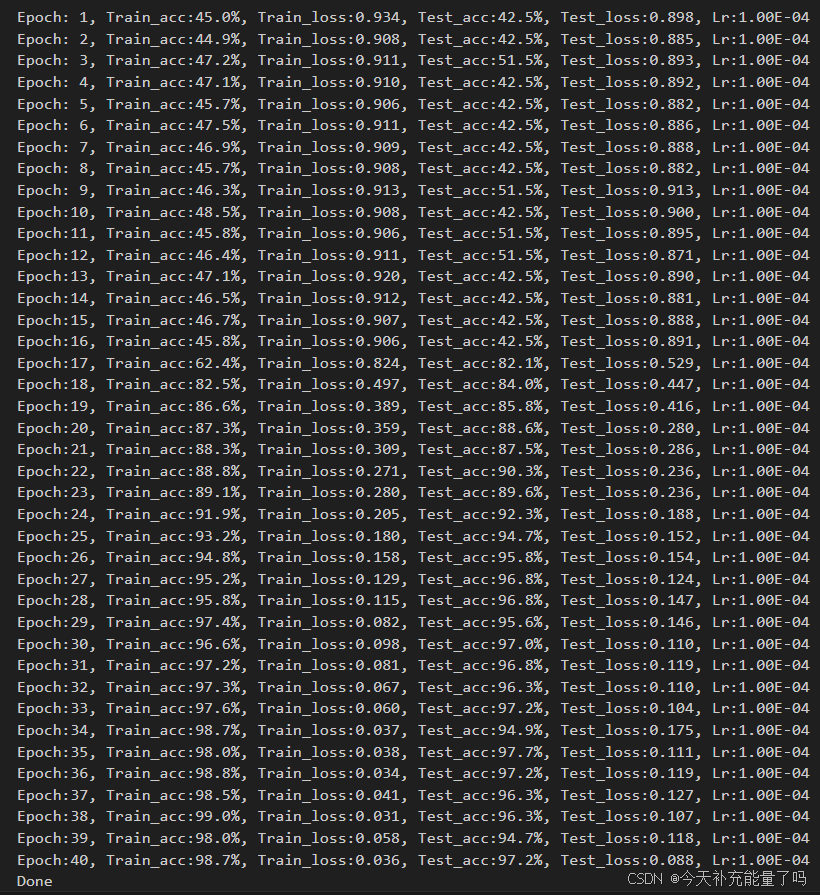
四、 结果可视化
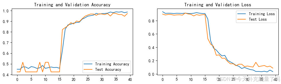
1. Loss与Accuracy图
# Plot the training and test loss
epochs_range = range(epochs)

plt.figure(figsize=(12, 3))
plt.subplot(1, 2, 1)

plt.plot(epochs_range, train_acc, label='Training Accuracy')
plt.plot(epochs_range, test_acc, label='Test Accuracy')
plt.legend(loc='lower right')
plt.title('Training and Validation Accuracy')

plt.subplot(1, 2, 2)
plt.plot(epochs_range, train_loss, label='Training Loss')
plt.plot(epochs_range, test_loss, label='Test Loss')
plt.legend(loc='upper right')
plt.title('Training and Validation Loss')
plt.show()
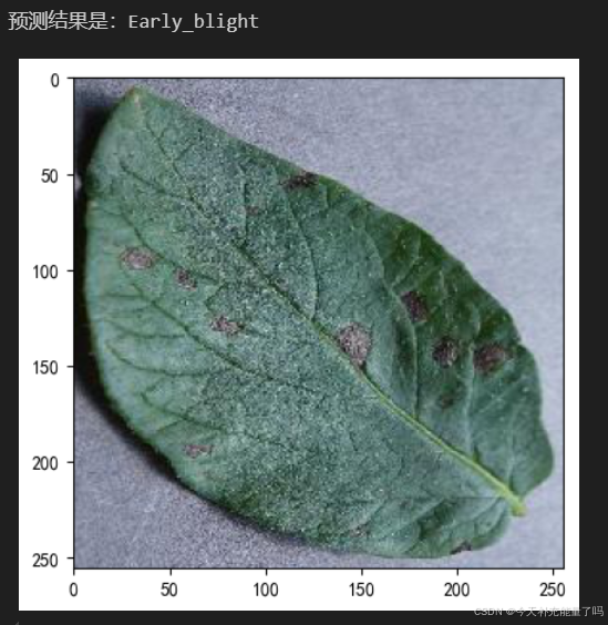
2. 指定图片进行预测
# Predict the class of an image
classes = list(total_data.class_to_idx)

def predict_one_image(image_path, model, transform, classes):


    test_img = Image.open(image_path).convert('RGB')
    plt.imshow(test_img)  # 展示预测的图片

    test_img = transform(test_img)
    img = test_img.to(device).unsqueeze(0)


    model.eval()
    output = model(img)

    _,pred = torch.max(output,1)
    pred_class = classes[pred]
    print(f'预测结果是:{pred_class}')

predict_one_image(image_path='./data/PotatoPlants/Early_blight/1.JPG',
                  model=model,
                  transform=train_transforms,
                  classes=classes)
3. 模型评估
# Evaluate the best model on the test set
best_model.eval()
epoch_test_acc, epoch_test_loss = test(test_dl, best_model, loss_fn)

epoch_test_acc, epoch_test_loss![]()


 被折叠的 条评论
为什么被折叠?
被折叠的 条评论
为什么被折叠?
 到【灌水乐园】发言


