斯坦福ML课程——python转写(Week2—课程作业ex1_2)

利用python完成课程作业ex1的第二部分，第二部分要求如下：

In this part, you will implement linear regression with multiple variables to predict the prices of houses. Suppose you are selling your house and you want to know what a good market price would be. One way to do this is to rst collect information on recent houses sold and make a model of housing prices.

在ex1_mul.py的代码中，分为三个部分，每个部分分别如下：

• Part 1: Feature Normalization
• Part 2: Gradient Descent
• Part 3: Normal Equations

具体代码如下：

# -*- coding: utf-8 -*-
"""
Created on Sun Nov 17 12:02:43 2019

@author: Lonely_hanhan
"""
import numpy as np
import matplotlib.pyplot as plt
from mpl_toolkits.mplot3d import Axes3D

print('Plotting Data ...\n')
Data = np.loadtxt('D:\exercise\machine-learning-ex1\machine-learning-ex1\ex1\ex1data2.txt', delimiter=',')
X = Data[:, [0, 1]]
[m,n] = X.shape
y = Data[:, 2]
y = y.reshape((m,1))

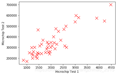
def PlotData(x, y):
     plt.plot(x[:,0], y, color='red', linewidth='2', marker='x', markersize='10', markerfacecolor = 'red', linestyle='None')
     plt.xlabel('Microchip Test 1')
     plt.ylabel('Microchip Test 2')

PlotData(X, y)
plt.show()
'''================ Part 1: Feature Normalization==============='''
# Print out some data points
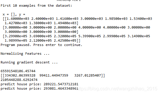
print('First 10 examples from the dataset: \n');
print(' x = [], y =  \n', np.array(np.hstack((X[1:10,:],y[1:10,:]))).T)
print('Program paused. Press enter to continue.\n')

#Scale features and set them to zero mean
print('Normalizing Features ...\n')

def featureNormalize(X):
    X_norm = X
    mu = np.zeros((1, X.shape[1]))
    sigma = np.zeros((1, X.shape[1]))
    mu = np.mean(X, axis = 0)
    sigma = np.std(X, axis = 0)
    X_norm = (X - mu)/sigma
    return X_norm, mu, sigma

[X,mu,sigma] = featureNormalize(X)

# Add intercept term to X

x_0 = np.ones((m , 1))
X = np.hstack((x_0 , X)) # Add a column of ones to X

'''================ Part 2: Gradient Descent ==============='''
print('Running gradient descent ...\n')

#Choose some alpha value
alpha = 0.01
num_iters = 400

#Init Theta and Run Gradient Descent
theta = np.zeros((1, 3))

def h_func(theta, X):
    return np.dot(X, theta.T)

def computeCostMulti(X, y, theta):
    m = len(y)
    J = 0
    J = np.sum(np.square((h_func(theta, X) - y))) / (2 * m)
    return J

def gradientDescentMulti(X, y, theta, alpha, num_iters):
    m = len(y)
    J_history = np.zeros((num_iters, 1))
    for iter1 in range(0, num_iters):
        theta = theta - alpha * np.dot((h_func(theta, X)-y).T, X) / m
        J_history[iter1] = computeCostMulti(X, y, theta)
    return theta, J_history

J = computeCostMulti(X, y, theta)
print(J)

[theta, J_history] = gradientDescentMulti(X, y, theta, alpha, num_iters)
print(theta)

J = computeCostMulti(X, y, theta)
print(J)
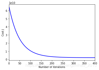
#Plot the convergence graph
N_f_itera = np.arange(1,len(J_history)+1)
plt.plot(N_f_itera, J_history, color='blue', linewidth='2', linestyle='-')
plt.ylim((0, 8*pow(10,10)))
plt.xlabel('Number of iterations')
plt.ylabel('Cost J')

def test(means, stds, theta):

    t1 = np.array([[1650,3]])

    t1 = t1 - means
    t1 = t1 / stds
    t1 = np.hstack((np.ones((t1.shape[0], 1)), t1))

    res = np.dot(t1, theta.T)
    print('predict house price:', res[0][0])

test(mu, sigma, theta)

'''================ Part 3: Normal Equations ==============='''

def normalEqn(X, y):
    theta = np.zeros((X.shape[1], 1))
    theta = np.dot(np.dot(np.linalg.inv(np.dot(X.T,X)), X.T),y)
    return theta
theta_nor = normalEqn(X, y)

test(mu, sigma, theta_nor.T)
    

 运行结果如下：

 

 

 为了记录自己的学习进度同时也加深自己对知识的认知，刚刚开始写博客，如有错误或者不妥之处，请大家给予指正。