


强化学习笔记
主要基于b站西湖大学赵世钰老师的【强化学习的数学原理】课程,个人觉得赵老师的课件深入浅出,很适合入门.
第一章 强化学习基本概念
第二章 贝尔曼方程
第三章 贝尔曼最优方程
第四章 值迭代和策略迭代
第五章 强化学习实例分析:GridWorld
第六章 蒙特卡洛方法
第七章 Robbins-Monro算法
第八章 多臂老虎机
第九章 强化学习实例分析:CartPole
文章目录
在强化学习实例分析:CartPole中,我们通过实验发现了蒙特卡洛方法的一些缺点:
- 每次更新需要等到一个episode结束;
- 越到后面的episode,耗时越长,效率低.
本节介绍强化学习中经典的时序差分方法(Temporal Difference Methods,TD)及其Python实现。与蒙特卡洛(MC)学习类似,TD学习也是Model-free的,但由于其增量形式在效率上相较于MC方法具有一定的优势。
一、on-policy vs off-policy
在介绍时序差分算法之前,首先介绍一下on-policy 和 off-policy的概念:
- On-policy:我们把用于产生采样样本的策略称为behavior-policy,在policy-improvement步骤进行改进的策略称为target-policy.如果这两个策略相同,我们称之为On-policy算法。
- Off-policy:如果behavior-policy和target-policy不同,我们称之为Off-policy算法。
比如在Monte-Carlo算法中,我可以用一个给定策略 π a \pi_a πa来产生样本,这个策略可以是 ϵ \epsilon ϵ-greedy策略,以保证能够访问所有的 s s s和 a a a。而我们目标策略可以是greedy策略 π b \pi_b πb,在policy-imporvement阶段我们不断改进 π b \pi_b πb,最终得到一个最优的策略。这样我们最后得到的最优策略 π b ∗ \pi_b^* πb∗就是一个贪婪策略,不用去探索不是最优的动作,这样我们用 π b ∗ \pi_b^* πb∗可以得到更高的回报。
二、TD learning of state values
1 迭代格式
和蒙特卡洛方法一样,用TD learning来估计状态值
v
(
s
)
v(s)
v(s),我们也需要采样的数据,假设给定策略
π
\pi
π,某个episode采样得到的序列如下:
(
s
0
,
r
1
,
s
1
,
.
.
.
,
s
t
,
r
t
+
1
,
s
t
+
1
,
.
.
.
)
(s_0, r_1, s_1, . . . , s_t , r_{t+1}, s_{t+1}, . . .)
(s0,r1,s1,...,st,rt+1,st+1,...)
那么TD learning给出在第
t
t
t步状态值
v
(
s
)
v(s)
v(s)的更新如下:
v
(
s
t
)
=
v
(
s
t
)
+
α
t
(
s
t
)
[
r
t
+
1
+
γ
v
(
s
t
+
1
)
−
v
(
s
t
)
]
(
1
)
v(s_t)=v(s_t)+\alpha_t(s_t)[r_{t+1}+\gamma v(s_{t+1})-v(s_t)]\qquad(1)
v(st)=v(st)+αt(st)[rt+1+γv(st+1)−v(st)](1)
Note:
- s t s_t st是当前状态, s t + 1 s_{t+1} st+1是跳转到的下一个状态,这里需要用到 v ( s t + 1 ) v(s_{t+1}) v(st+1)(本身也是一个估计值);
- 我们可以看到,TD方法在每个时间步都会进行更新,不需要得到整个episode结束才更新;
- 这个算法被称为TD(0)。
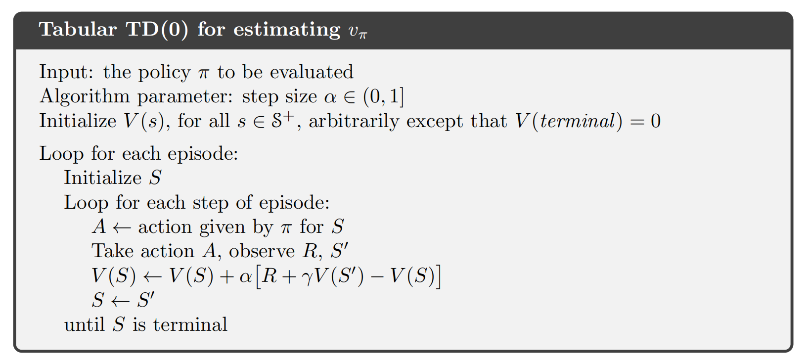
当 a t ( s t ) a_t(s_t) at(st)取常量 α \alpha α时,下面给出 v π ( s ) v_{\pi}(s) vπ(s)估计的伪代码:
2 推导
TD(0)的迭代格式为什么是这样的呢?和前面介绍随机近似中的RM算法似乎有点像,事实上它可以看作是求解Bellman方程的一种特殊的随机近似算法。我们回顾贝尔曼方程中介绍的:
v
π
(
s
)
=
E
[
G
t
∣
S
t
=
s
]
=
E
[
R
t
+
γ
G
t
+
1
∣
S
t
=
s
]
=
E
[
R
t
+
γ
v
π
(
S
t
+
1
)
∣
S
t
=
s
]
(
2
)
\begin{aligned} v_{\pi}(s)&=\mathbb{E}[G_t|S_t=s]\\ &=\mathbb{E}[R_t+\gamma G_{t+1}|S_t=s]\\ &=\mathbb{E}[R_t+\gamma v_{\pi}(S_{t+1})|S_t=s]\\ \end{aligned} \qquad(2)
vπ(s)=E[Gt∣St=s]=E[Rt+γGt+1∣St=s]=E[Rt+γvπ(St+1)∣St=s](2)
下面我们用Robbins-Monro算法来求解方程(2),对于状态$s_t, $,我们定义一个函数为
g
(
v
π
(
s
t
)
)
≐
v
π
(
s
t
)
−
E
[
R
t
+
1
+
γ
v
π
(
S
t
+
1
)
∣
S
t
=
s
t
]
.
g(v_\pi(s_t))\doteq v_\pi(s_t)-\mathbb{E}\big[R_{t+1}+\gamma v_\pi(S_{t+1})|S_t=s_t\big].
g(vπ(st))≐vπ(st)−E[Rt+1+γvπ(St+1)∣St=st].
那么方程(2)等价于
g
(
v
π
(
s
t
)
)
=
0.
g(v_\pi(s_t))=0.
g(vπ(st))=0.
显然我们可以用RM算法来求解上述方程的根,就能得到
v
π
(
s
t
)
v_{\pi}(s_t)
vπ(st)。因为我们可以通过采样获得
r
t
+
1
r_{t+1}
rt+1和
s
t
+
1
s_{t+1}
st+1,它们是
R
t
+
1
R_{t+1}
Rt+1和
S
t
+
1
S_{t+ 1}
St+1的样本,我们可以获得的$g( v_\pi ( s_{t}) ) $的噪声观测是
g
~
(
v
π
(
s
t
)
)
=
v
π
(
s
t
)
−
[
r
t
+
1
+
γ
v
π
(
s
t
+
1
)
]
=
(
v
π
(
s
t
)
−
E
[
R
t
+
1
+
γ
v
π
(
S
t
+
1
)
∣
S
t
=
s
t
]
)
⏟
g
(
v
π
(
s
t
)
)
+
(
E
[
R
t
+
1
+
γ
v
π
(
S
t
+
1
)
∣
S
t
=
s
t
]
−
[
r
t
+
1
+
γ
v
π
(
s
t
+
1
)
]
)
⏟
η
.
\begin{aligned}\tilde{g}(v_{\pi}(s_{t}))&=v_\pi(s_t)-\begin{bmatrix}r_{t+1}+\gamma v_\pi(s_{t+1})\end{bmatrix}\\&=\underbrace{\left(v_\pi(s_t)-\mathbb{E}\big[R_{t+1}+\gamma v_\pi(S_{t+1})|S_t=s_t\big]\right)}_{g(v_\pi(s_t))}\\&+\underbrace{\left(\mathbb{E}\big[R_{t+1}+\gamma v_\pi(S_{t+1})|S_t=s_t\big]-\big[r_{t+1}+\gamma v_\pi(s_{t+1})\big]\right)}_{\eta}.\end{aligned}
g~(vπ(st))=vπ(st)−[rt+1+γvπ(st+1)]=g(vπ(st))
(vπ(st)−E[Rt+1+γvπ(St+1)∣St=st])+η
(E[Rt+1+γvπ(St+1)∣St=st]−[rt+1+γvπ(st+1)]).
因此,求解
g
(
v
π
(
s
t
)
)
=
0
g(v_{\pi}(s_{t}))=0
g(vπ(st))=0的RM算法为
v
t
+
1
(
s
t
)
=
v
t
(
s
t
)
−
α
t
(
s
t
)
g
~
(
v
t
(
s
t
)
)
=
v
t
(
s
t
)
−
α
t
(
s
t
)
(
v
t
(
s
t
)
−
[
r
t
+
1
+
γ
v
π
(
s
t
+
1
)
]
)
,
(
3
)
\begin{aligned}v_{t+1}(s_{t})&=v_t(s_t)-\alpha_t(s_t)\tilde{g}(v_t(s_t))\\&=v_t(s_t)-\alpha_t(s_t)\Big(v_t(s_t)-\big[r_{t+1}+\gamma v_\pi(s_{t+1})\big]\Big),\end{aligned}\qquad(3)
vt+1(st)=vt(st)−αt(st)g~(vt(st))=vt(st)−αt(st)(vt(st)−[rt+1+γvπ(st+1)]),(3)
其中
v
t
(
s
t
)
v_t(s_t)
vt(st)是
v
π
(
s
t
)
v_\pi(s_t)
vπ(st)在
t
t
t时间点的估计,
α
t
(
s
t
)
\alpha_t(s_t)
αt(st)是学习率。
Note:
- (3)中的算法与(1)中的TD(0)具有相似的表达式,唯一的区别是(3)的右侧包含 v π ( s t + 1 ) v_{\pi}(s_{t+1}) vπ(st+1),而(1)包含 v t ( s t + 1 ) v_t(s_{t+1}) vt(st+1),这是因为(3)的设计是通过假设其他状态值已知来估计 s t s_t st的动作值。
- 如果我们想估计所有状态的状态值,则右侧的 v π ( s t + 1 ) v_{\pi}(s_{t+1}) vπ(st+1)应替换为 v t ( s t + 1 ) v_t(s_{t+1}) vt(st+1),那么(3)与(1)完全相同。并且我们可以证明这样的替换能保证所有 v t ( s ) v_t(s) vt(s)都收敛到 v π ( s ) v_{\pi}(s) vπ(s),这里就不再展开。
3 分析
我们再来看一下TD(0)的迭代格式:
v
t
+
1
(
s
t
)
⏟
new estimate
=
v
t
(
s
t
)
⏟
current estimate
−
α
t
(
s
t
)
[
v
t
(
s
t
)
−
(
r
t
+
1
+
γ
v
t
(
s
t
+
1
)
⏟
TD target
v
ˉ
t
)
⏞
TD error
δ
t
]
,
(
4
)
\underbrace{v_{t+1}(s_t)}_{\text{new estimate}}=\underbrace{v_t(s_t)}_{\text{current estimate}}-\alpha_t(s_t)\Big[\overbrace{v_t(s_t)-\Big(\underbrace{r_{t+1}+\gamma v_t(s_{t+1})}_{\text{TD target }\bar{v}_t}\Big)}^{\text{TD error }\delta_t}\Big],\qquad (4)
new estimate
vt+1(st)=current estimate
vt(st)−αt(st)[vt(st)−(TD target vˉt
rt+1+γvt(st+1))
TD error δt],(4)
其中
v
ˉ
t
≐
r
t
+
1
+
γ
v
t
(
s
t
+
1
)
(
5
)
\bar{v}_t\doteq r_{t+1}+\gamma v_t(s_{t+1})\qquad(5)
vˉt≐rt+1+γvt(st+1)(5)
被称为TD target,
δ
t
≐
v
(
s
t
)
−
v
ˉ
t
=
v
t
(
s
t
)
−
(
r
t
+
1
+
γ
v
t
(
s
t
+
1
)
)
(
6
)
\delta_t\doteq v(s_t)-\bar{v}_t=v_t(s_t)-(r_{t+1}+\gamma v_t(s_{t+1}))\qquad(6)
δt≐v(st)−vˉt=vt(st)−(rt+1+γvt(st+1))(6)
被称为TD-error.
为什么(5)被称为TD target,因为迭代格式(4)是让
v
t
+
1
v_{t+1}
vt+1朝着
v
ˉ
t
\bar{v}_t
vˉt更新的,我们考察:
∣
v
t
+
1
(
s
t
)
−
v
ˉ
t
∣
=
∣
[
v
t
(
s
t
)
−
v
ˉ
t
]
−
α
t
(
s
t
)
[
v
t
(
s
t
)
−
v
ˉ
t
]
∣
=
∣
[
1
−
α
t
(
s
t
)
]
∣
∣
[
v
t
(
s
t
)
−
v
ˉ
t
]
∣
≤
∣
[
v
t
(
s
t
)
−
v
ˉ
t
]
∣
\begin{aligned} |v_{t+1}(s_t)-\bar{v}_t|&=|\begin{bmatrix}v_t(s_t)-\bar{v}_t\end{bmatrix}-\alpha_t(s_t)\big[v_t(s_t)-\bar{v}_t\big]|\\ &=|[1-\alpha_t(s_t)]||\big[v_t(s_t)-\bar{v}_t\big]|\\ &\leq|\big[v_t(s_t)-\bar{v}_t\big]| \end{aligned}
∣vt+1(st)−vˉt∣=∣[vt(st)−vˉt]−αt(st)[vt(st)−vˉt]∣=∣[1−αt(st)]∣∣[vt(st)−vˉt]∣≤∣[vt(st)−vˉt]∣
显然当
0
<
α
t
(
s
t
)
<
2
0<\alpha_t(s_t)<2
0<αt(st)<2时,上式的不等式成立,这意味着
v
t
+
1
v_{t+1}
vt+1比
v
t
v_t
vt离
v
ˉ
t
\bar{v}_t
vˉt更近,所以
v
ˉ
t
\bar{v}_t
vˉt被称为TD target。
TD-error则衡量了在
t
t
t时间步估计值
v
t
v_t
vt与
v
ˉ
t
\bar{v}_t
vˉt 的差异,显然我们可以想象当
v
t
v_t
vt估计值是准确的
v
π
v_{\pi}
vπ时,TD-error的期望值应该为0,事实上确实如此:
E
[
δ
t
∣
S
t
=
s
t
]
=
E
[
v
π
(
S
t
)
−
(
R
t
+
1
+
γ
v
π
(
S
t
+
1
)
)
∣
S
t
=
s
t
]
=
v
π
(
s
t
)
−
E
[
R
t
+
1
+
γ
v
π
(
S
t
+
1
)
∣
S
t
=
s
t
]
=
v
π
(
s
t
)
−
v
π
(
s
t
)
=
0.
\begin{aligned} \mathbb{E}[\delta_t|S_t=s_t]& =\mathbb{E}\big[v_\pi(S_t)-(R_{t+1}+\gamma v_\pi(S_{t+1}))|S_t=s_t\big] \\ &=v_\pi(s_t)-\mathbb{E}\big[R_{t+1}+\gamma v_\pi(S_{t+1})|S_t=s_t\big] \\ &=v_\pi(s_t)-v_\pi(s_t)\\ &=0. \end{aligned}
E[δt∣St=st]=E[vπ(St)−(Rt+1+γvπ(St+1))∣St=st]=vπ(st)−E[Rt+1+γvπ(St+1)∣St=st]=vπ(st)−vπ(st)=0.
当TD-error趋于0时, 那么(1)也得到不到什么新的信息了,迭代也就收敛了。
4 TD(0)与蒙特卡洛方法的对比
| TD learning | Monte Carlo Methods |
|---|---|
| TD learning每得到一个样本就能更新 v ( s ) v(s) v(s)或者 q ( s , a ) q(s,a) q(s,a),这种算法被称为online的. | MC每次更新必须等到一个epsisode结束,这种算法被称为offline的. |
| TD可以处理连续性任务和episodic任务. | MC只能处理episodic任务. |
| TD被称为bootstraping方法,因为 v ( s ) v(s) v(s)/ q ( s , a ) q(s,a) q(s,a)动作的更新依赖于其他状态值先前的估计值.因此,TD需要给定一个初始值. | MC是Non-Bootstraping的. |
三、Sarsa
如果我们要得到最优策略,无论是用策略迭代还是值迭代算法,我们都需要
q
(
s
,
a
)
q(s,a)
q(s,a),所以我们可以用TD learning直接来估计
q
(
s
,
a
)
q(s,a)
q(s,a),给定策略
π
\pi
π,假设某个episode采样得到如下序列:
(
s
0
,
a
0
,
r
1
,
s
1
,
a
1
,
.
.
.
,
s
t
,
a
t
,
r
t
+
1
,
s
t
+
1
,
a
t
+
1
,
.
.
.
)
.
(s_0, a_0, r_1, s_1, a_1, . . . , s_t , a_t , r_{t+1}, s_{t+1}, a_{t+1}, . . .).
(s0,a0,r1,s1,a1,...,st,at,rt+1,st+1,at+1,...).
那么TD learning对
q
(
s
,
a
)
q(s,a)
q(s,a)的估计如下:
q
t
+
1
(
s
t
,
a
t
)
=
q
t
(
s
t
,
a
t
)
−
α
t
(
s
t
,
a
t
)
[
q
t
(
s
t
,
a
t
)
−
(
r
t
+
1
+
γ
q
t
(
s
t
+
1
,
a
t
+
1
)
)
]
,
(
7
)
q_{t+1}(s_t,a_t)=q_t(s_t,a_t)-\alpha_t(s_t,a_t)\Big[q_t(s_t,a_t)-(r_{t+1}+\gamma q_t(s_{t+1},a_{t+1}))\Big],\qquad(7)
qt+1(st,at)=qt(st,at)−αt(st,at)[qt(st,at)−(rt+1+γqt(st+1,at+1))],(7)
Note:
- 和对状态值的估计(1)对比,我们发现(7)就是把(1)中的 v ( s ) v(s) v(s)替换为 q ( s , a ) q(s,a) q(s,a),其实就是用RM算法求解关于 q ( s , a ) q(s,a) q(s,a)的贝尔曼方程,所以得到的迭代格式类似.
- 其中 s t + 1 s_{t+1} st+1为转移的下一个状态, a t + 1 a_{t+1} at+1是在状态 s t + 1 s_{t+1} st+1下采取的动作,这里是根据策略 π \pi π得到.(因为我们采样的序列就是根据 π \pi π得到的)
- 所以如果 s t + 1 s_{t+1} st+1是终止状态,显然就没有 a t + 1 a_{t+1} at+1,此时我们定义 q ( s t + 1 , a t + 1 ) = 0 q(s_{t+1},a_{t+1})=0 q(st+1,at+1)=0.
- 这个算法每次更新会用到
(
s
t
,
a
t
,
r
t
+
1
,
s
t
+
1
,
a
t
+
1
)
(s_t, a_t, r_{t+1}, s_{t+1}, a_{t+1})
(st,at,rt+1,st+1,at+1)(SARSA),所以这个算法被称为
SARSA. - 当我们有 q ( s , a ) q(s,a) q(s,a)的估计值后,我们可以使用greedy或者 ε \varepsilon ε-greedy来更新策略。可以证明如果步长 a t ( s t , a t ) a_t(s_t,a_t) at(st,at)满足RM算法收敛的条件要求,只要所有的状态-动作对被访问无限次,Sarsa以概率1收敛到最优的策略 π ∗ \pi^* π∗和最优的动作-价值函数 q ∗ ( s , a ) q^*(s,a) q∗(s,a).
同TD(0)类似,Sarsa可以看作是用RM算法求解如下贝尔曼方程得到的迭代格式:
q
π
(
s
,
a
)
=
E
[
R
+
γ
q
π
(
S
′
,
A
′
)
∣
s
,
a
]
,
for all
(
s
,
a
)
.
q_\pi(s,a)=\mathbb{E}\left[R+\gamma q_\pi(S',A')|s,a\right],\quad\text{for all }(s,a).
qπ(s,a)=E[R+γqπ(S′,A′)∣s,a],for all (s,a).
下面给出Sarsa完整的伪代码:
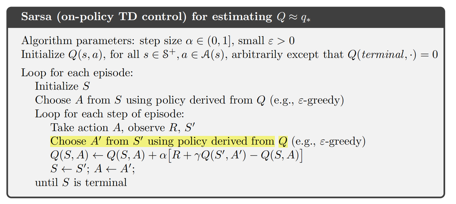
Sarsa是一种on-policy算法,因为在估计 q t q_t qt值时,会用到依据 π t \pi_t πt产生的样本,更新 q t q_t qt后,我们又会依据新的 q t q_t qt来更新策略得到 π t + 1 \pi_{t+1} πt+1,然后用 π t + 1 \pi_{t+1} πt+1产生样本继续更新 q t + 1 q_{t+1} qt+1,这样交替进行,最后得到最优策略。在这个过程中我们发现产生样本的策略和得到的最优策略是同一个策略,所以是on-policy算法。
四、Expected Sarsa
给定策略
π
\pi
π,其动作值可以用Sarsa的一种变体Expected-Sarsa来估计。Expected-Sarsa的迭代格式如下:
q
t
+
1
(
s
t
,
a
t
)
=
q
t
(
s
t
,
a
t
)
−
α
t
(
s
t
,
a
t
)
[
q
t
(
s
t
,
a
t
)
−
(
r
t
+
1
+
γ
E
[
q
t
(
s
t
+
1
,
A
)
]
)
]
=
q
t
(
s
t
,
a
t
)
−
α
t
(
s
t
,
a
t
)
[
q
t
(
s
t
,
a
t
)
−
(
r
t
+
1
+
γ
∑
a
π
(
a
∣
s
t
+
1
)
q
t
(
s
t
+
1
)
,
a
)
]
\begin{aligned} q_{t+1}(s_t,a_t)&=q_t(s_t,a_t)-\alpha_t(s_t,a_t)\Big[q_t(s_t,a_t)-(r_{t+1}+\gamma\mathbb{E}[q_t(s_{t+1},A)])\Big]\\ &=q_t(s_t,a_t)-\alpha_t(s_t,a_t)\Big[q_t(s_t,a_t)-(r_{t+1}+\gamma\sum_a\pi(a|s_{t+1})q_t(s_{t+1}),a)\Big] \end{aligned}
qt+1(st,at)=qt(st,at)−αt(st,at)[qt(st,at)−(rt+1+γE[qt(st+1,A)])]=qt(st,at)−αt(st,at)[qt(st,at)−(rt+1+γa∑π(a∣st+1)qt(st+1),a)]
同Sarsa类似,Expected-Sarsa可以看作是用RM算法求解如下贝尔曼方程得到的迭代格式:
q
π
(
s
,
a
)
=
E
[
R
t
+
1
+
γ
E
[
q
π
(
S
t
+
1
,
A
t
+
1
)
∣
S
t
+
1
]
∣
S
t
=
s
,
A
t
=
a
]
=
E
[
R
t
+
1
+
γ
v
π
(
S
t
+
1
)
∣
S
t
=
s
,
A
t
=
a
]
.
\begin{aligned} q_\pi(s,a)&=\mathbb{E}\Big[R_{t+1}+\gamma\mathbb{E}[q_\pi(S_{t+1},A_{t+1})|S_{t+1}]\Big|S_t=s,A_t=a\Big]\\ &=\mathbb{E}\Big[R_{t+1}+\gamma v_\pi(S_{t+1})|S_t=s,A_t=a\Big]. \end{aligned}
qπ(s,a)=E[Rt+1+γE[qπ(St+1,At+1)∣St+1]
St=s,At=a]=E[Rt+1+γvπ(St+1)∣St=s,At=a].
虽然Expected Sarsa的计算复杂度比Sarsa高,但它消除了随机选择
a
t
+
1
a_{t+1}
at+1所带来的方差。在相同的采样样本条件下,Expected Sarsa的表现通常比Sarsa更好。
五、Q-learning
接下来我们介绍强化学习中经典的Q-learning算法,Sarsa算法和Expected-Sarsa都是估计
q
(
s
,
a
)
q(s,a)
q(s,a),如果我们想要得到最优策略还需要policy-improvement,而Q-learning算法则是直接估计
q
∗
(
s
,
a
)
q^*(s,a)
q∗(s,a),如果我们能得到
q
∗
(
s
,
a
)
q^*(s,a)
q∗(s,a)就不用每一步还执行policy-improvement了。Q-learning的迭代格式如下:
q
t
+
1
(
s
t
,
a
t
)
=
q
t
(
s
t
,
a
t
)
−
α
t
(
s
t
,
a
t
)
[
q
t
(
s
t
,
a
t
)
−
(
r
t
+
1
+
γ
max
a
∈
A
(
s
t
+
1
)
q
t
(
s
t
+
1
,
a
)
)
]
,
(
7.18
)
q_{t+1}(s_t,a_t)=q_t(s_t,a_t)-\alpha_t(s_t,a_t)\left[q_t(s_t,a_t)-\left(r_{t+1}+\gamma\max_{a\in\mathcal{A}(s_{t+1})}q_t(s_{t+1},a)\right)\right],\quad(7.18)
qt+1(st,at)=qt(st,at)−αt(st,at)[qt(st,at)−(rt+1+γa∈A(st+1)maxqt(st+1,a))],(7.18)
Q-learning也是一种随机近似算法,用于求解以下方程:
q
(
s
,
a
)
=
E
[
R
t
+
1
+
γ
max
a
q
(
S
t
+
1
,
a
)
∣
S
t
=
s
,
A
t
=
a
]
.
q(s,a)=\mathbb{E}\left[R_{t+1}+\gamma\max_aq(S_{t+1},a)\Big|S_t=s,A_t=a\right].
q(s,a)=E[Rt+1+γamaxq(St+1,a)
St=s,At=a].
这是
q
(
s
,
a
)
q(s,a)
q(s,a)贝尔曼最优方程,所以Q-learning本质就是求解贝尔曼最优方程的随机近似算法,其伪代码如下:
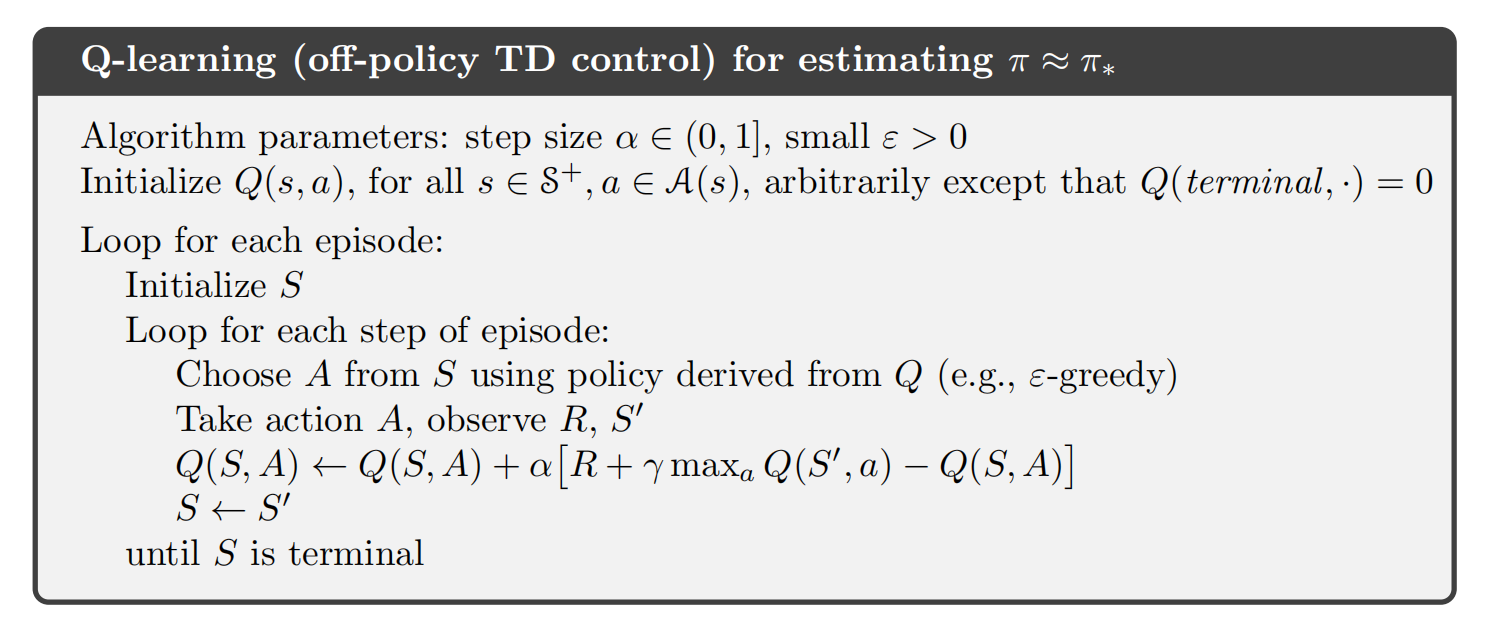
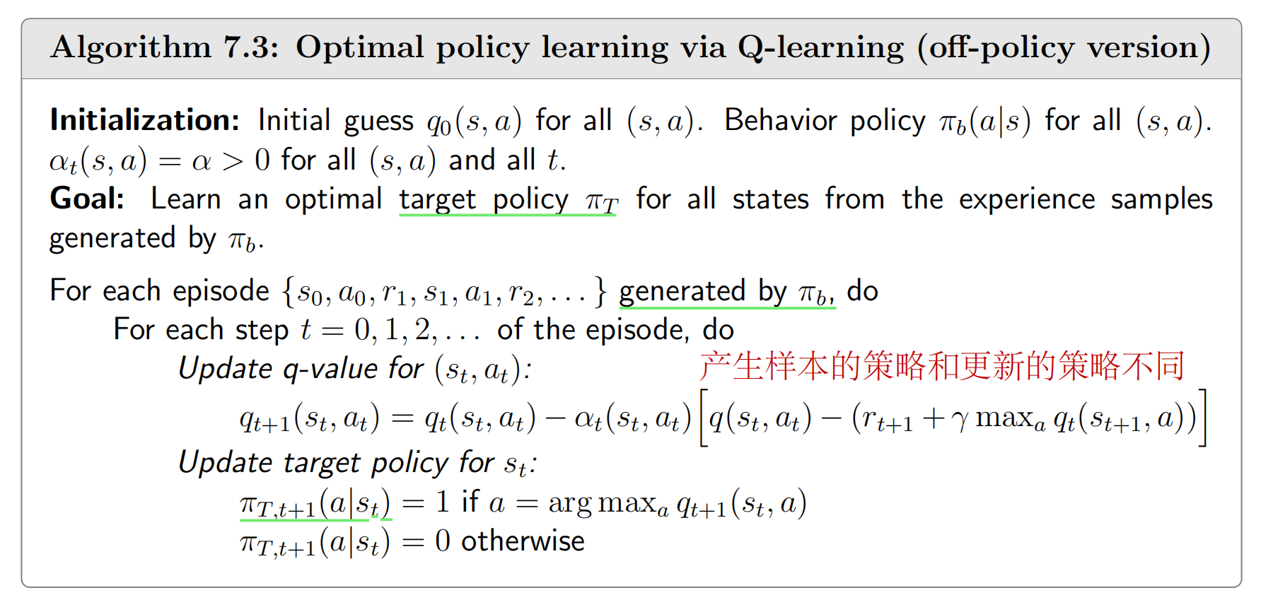
显然Q-learning是一种Off-policy算法,因为 q t ( s , a ) q_t(s,a) qt(s,a)在更新的时候,用的数据可以是一个给定 ϵ \epsilon ϵ-greedy策略 π a \pi_a πa产生的,但是直接学习到 q ∗ ( s , a ) q^*(s,a) q∗(s,a),我们可以通过 q ∗ ( s , a ) q^*(s,a) q∗(s,a)得到一个greedy策略 π b ∗ \pi_b^* πb∗.
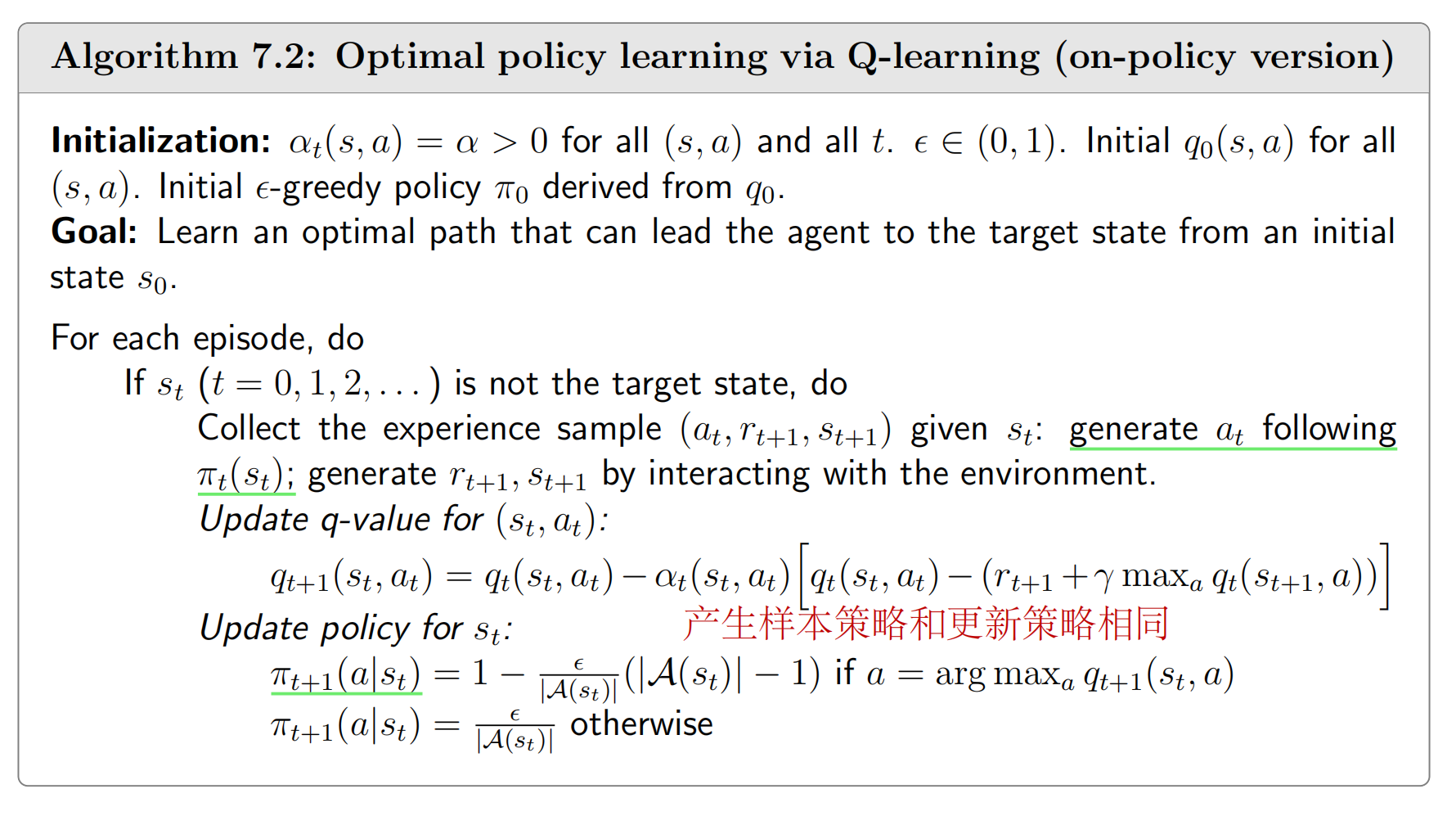
即使Q-learning是off-policy的,但我们也可以按on-policy的方式来实现,下面给出这两种实现,我们可以更清楚地看到off-policy和on-policy的区别:
六、Python实现
1 Cliff Walking问题描述
在本节中,我们使用SARSA和Q-learning算法来解决Cliff Walking问题。(参见Sutton&Barto例6.6)
如下图所示,黑色格子代表墙壁/障碍物,白色格子代表非终点格子,带有“s”的格子是每个episode的起点,带有“G”的格子是目标点。
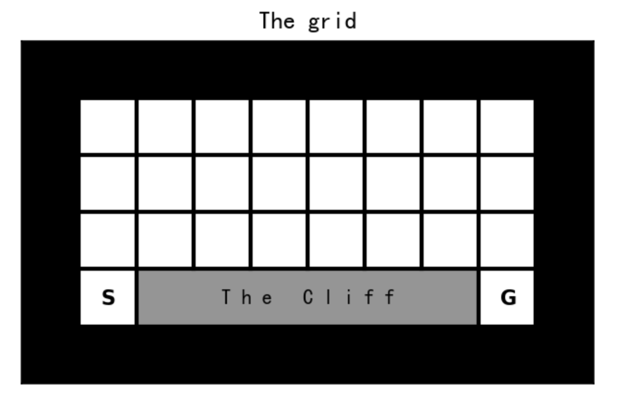
智能体从“s”格子开始。在每一步中,智能体可以选择四种操作中的一种:“上”、“右”、“下”、“左”,移动到该方向的下一个格子。
- 如果下一个格子是墙/障碍物,智能体不会移动,并获得-1奖励;
- 如果下一个格子是一个非终端格子,智能体移动到该格子并获得-1奖励;
- 如果下一个格子是目标格子,则该episode结束,智能体将获得100奖励(设置为100以加速训练);
- 如果下一个格子是悬崖,则该episode结束,智能体将获得-100奖励.
我们在GridWorld类实现了这个环境以及智能体与环境的交互操作,代码如下,文件命名为gridworld.py:
import matplotlib.pyplot as plt
import numpy as np


class GridWorld:

    def __init__(self, reward_wall=-1):
        # initialize grid with 2d numpy array
        # >0: goal
        # -1: wall/obstacles
        # 0: non-terminal
        self._grid = np.array(
            [ [0, 0, 0, 0, 0, 0, 0, 0],
             [0, 0, 0, 0, 0, 0, 0, 0],
             [0, 0, 0, 0, 0, 0, 0, 0],
             [0, -100, -100, -100, -100, -100, -100, 100]
             ])
        # wall around the grid, padding grid with -1
        self._grid_padded = np.pad(self._grid, pad_width=1, mode='constant', constant_values=-1)
        self._reward_wall = reward_wall

        # set start state
        self._start_state = (3, 0)
        self._random_start = False

        # store position of goal states and non-terminal states
        idx_goal_state_y, idx_goal_state_x = np.nonzero(self._grid > 0)
        self._goal_states = [(idx_goal_state_y[i], idx_goal_state_x[i]) for i in range(len(idx_goal_state_x))]

        idx_non_term_y, idx_non_term_x = np.nonzero(self._grid == 0)
        self._non_term_states = [(idx_non_term_y[i], idx_non_term_x[i]) for i in range(len(idx_non_term_x))]

        # store the current state in the padded grid
        self._state_padded = (self._start_state[0] + 1, self._start_state[1] + 1)

    def get_state_num(self):
        # get the number of states (total_state_number) in the grid, note: the wall/obstacles inside the grid are
        # counted as state as well
        return np.prod(np.shape(self._grid))

    def get_state_grid(self):

        state_grid = np.multiply(np.reshape(np.arange(self.get_state_num()), self._grid.shape), self._grid >= 0) - (
                self._grid == -1) #- (self._grid == -100)

        return state_grid, np.pad(state_grid, pad_width=1, mode='constant', constant_values=-1)

    def get_current_state(self):
        # get the current state as an integer from 0 to total_state_number-1
        y, x = self._state_padded
        return (y - 1) * self._grid.shape[1] + (x - 1)

    def int_to_state(self, int_obs):
        # convert an integer from 0 to total_state_number-1 to the position on the non-padded grid
        x = int_obs % self._grid.shape[1]
        y = int_obs // self._grid.shape[1]
        return y, x

    def reset(self):
        # reset the gridworld
        if self._random_start:
            # randomly start at a non-terminal state
            idx_start = np.random.randint(len(self._non_term_states))
            start_state = self._non_term_states[idx_start]
            self._state_padded = (start_state[0] + 1, start_state[1] + 1)
        else:
            # start at the designated start_state
            self._state_padded = (self._start_state[0] + 1, self._start_state[1] + 1)

    def step(self, action):
        # take one step according to the action
        # input: action (integer between 0 and 3)
        # output: reward           reward of this action
        #         terminated       1 if reaching the terminal state, 0 otherwise
        #         next_state       next state after this action, integer from 0 to total_state_number-1)
        y, x = self._state_padded

        if action == 0:  # up
            new_state_padded = (y - 1, x)
        elif action == 1:  # right
            new_state_padded = (y, x + 1)
        elif action == 2:  # down
            new_state_padded = (y + 1, x)
        elif action == 3:  # left
            new_state_padded = (y, x - 1)
        else:
            raise ValueError("Invalid action: {} is not 0, 1, 2, or 3.".format(action))

        new_y, new_x = new_state_padded
        if self._grid_padded[new_y, new_x] == -1:  # wall/obstacle
            reward = self._reward_wall
            new_state_padded = (y, x)
        elif self._grid_padded[new_y, new_x] == 0:  # non-terminal cell
            reward = self._reward_wall
        else:  # a goal
            reward = self._grid_padded[new_y, new_x]
            self.reset()
            terminated = 1
            return reward, terminated, self.get_current_state()

        terminated = 0
        self._state_padded = new_state_padded
        return reward, terminated, self.get_current_state()

    def plot_grid(self, plot_title=None):
        # plot the grid
        plt.figure(figsize=(5, 5),dpi=150)
        plt.imshow((self._grid_padded == -1) + (self._grid_padded == -100) * 0.5, cmap='Greys', vmin=0, vmax=1)
        ax = plt.gca()
        ax.grid(0)
        plt.xticks([])
        plt.yticks([])

        if plot_title:
            plt.title(plot_title)

        plt.text(
            self._start_state[1] + 1, self._start_state[0] + 1,
            r"$\mathbf{S}$", ha='center', va='center')
        for goal_state in self._goal_states:
            plt.text(
                goal_state[1] + 1, goal_state[0] + 1,
                r"$\mathbf{G}$", ha='center', va='center')
        h, w = self._grid_padded.shape
        for y in range(h - 1):
            plt.plot([-0.5, w - 0.5], [y + 0.5, y + 0.5], '-k', lw=2)
        for x in range(w - 1):
            if x in np.arange(2,7):
                plt.plot([x + 0.5, x + 0.5], [-0.5, h - 2.5], '-k', lw=2)
                continue
            plt.plot([x + 0.5, x + 0.5], [-0.5, h - 0.5], '-k', lw=2)
        plt.text(4.5, 4,r"T h e   C l i f f", ha='center', va='center')

    def plot_state_values(self, state_values, value_format="{:.1f}",plot_title=None):
        # plot the state values
        # input: state_values     (total_state_number, )-numpy array, state value function
        #        plot_title       str, title of the plot
        plt.figure(figsize=(5, 5),dpi=150)
        plt.imshow((self._grid_padded == -1) + (self._grid_padded == -100) * 0.5, cmap='Greys', vmin=0, vmax=1)
        ax = plt.gca()
        ax.grid(0)
        plt.xticks([])
        plt.yticks([])

        if plot_title:
            plt.title(plot_title)

        for (int_obs, state_value) in enumerate(state_values):
            y, x = self.int_to_state(int_obs)
            if (y, x) in self._non_term_states:
                plt.text(x + 1, y + 1, value_format.format(state_value), ha='center', va='center')
        for goal_state in self._goal_states:
            plt.text(
                goal_state[1] + 1, goal_state[0] + 1,
                r"$\mathbf{G}$", ha='center', va='center')
        h, w = self._grid_padded.shape
        for y in range(h - 1):
            plt.plot([-0.5, w - 0.5], [y + 0.5, y + 0.5], '-k', lw=2)
        for x in range(w - 1):
            if x in np.arange(2,7):
                plt.plot([x + 0.5, x + 0.5], [-0.5, h - 2.5], '-k', lw=2)
                continue
            plt.plot([x + 0.5, x + 0.5], [-0.5, h - 0.5], '-k', lw=2)

    def plot_policy(self, policy, plot_title=None):
        # plot a deterministic policy
        # input: policy           (total_state_number, )-numpy array, contains action as integer from 0 to 3
        #        plot_title       str, title of the plot
        action_names = [r"$\uparrow$", r"$\rightarrow$", r"$\downarrow$", r"$\leftarrow$"]
        plt.figure(figsize=(5, 5),dpi=150)
        plt.imshow((self._grid_padded == -1) + (self._grid_padded == -100) * 0.5, cmap='Greys', vmin=0, vmax=1)
        ax = plt.gca()
        ax.grid(0)
        plt.xticks([])
        plt.yticks([])

        for goal_state in self._goal_states:
            plt.text(
                goal_state[1] + 1, goal_state[0] + 1,
                r"$\mathbf{G}$", ha='center', va='center')

        if plot_title:
            plt.title(plot_title)

        for (int_obs, action) in enumerate(policy):
            y, x = self.int_to_state(int_obs)
            if (y, x) in self._non_term_states:
                action_arrow = action_names[action]
                plt.text(x + 1, y + 1, action_arrow, ha='center', va='center')
2 SARSA
下面我们实现了SARSA算法,可以看到其实很简单,就是把伪代码翻译过来就行:
def update_Q(Q, current_idx, next_idx, current_action, next_action, alpha, R, gamma, terminated):
    # Update Q at the each step
    #
    # input:  current Q,                    (array)
    #         current_idx, next_idx         (array)  states
    #         current_action, next_action   (array)  actions
    #         alpha, R, gamma               (floats) learning rate, reward, discount rate
    # output: Updated Q
    #
    if terminated:
        TD_error = R - Q[current_idx,current_action]
    else:
        TD_error = R + gamma*Q[next_idx,next_action] - Q[current_idx,current_action]
    Q[current_idx,current_action] = Q[current_idx,current_action] + alpha*TD_error

    return Q

def get_action(current_idx, Q, epsilon):

    # Choose optimal action based on current state and Q
    #
    # input:  current_idx     (array)
    #         Q,              (array)
    #         epsilon,        (float)
    # output: action

    action = np.argmax(Q[current_idx,:]) if np.random.rand() > epsilon else np.random.randint(4)

    return action
我们用SARSA算法来训练:
## SARSA

%matplotlib inline
import numpy as np
import matplotlib.pyplot as plt
from gridworld import GridWorld


Q  = np.zeros((25,4))
gw.reset()

max_ep = 5000

total_reward_sarsa = np.zeros(max_ep)

epsilon = 0.1
alpha = 0.6
gamma = 0.9


for ep in range(0, max_ep):
    gw.reset()
    terminated = False

    current_action = get_action(gw.get_current_state(),Q,epsilon)

    while terminated == False:
        reward, terminated, next_state = gw.step(current_action)

        if not reward == 100:
            total_reward_sarsa[ep] += reward

        next_action = get_action(next_state,Q,epsilon)

        Q = update_Q(Q, current_state, next_state, current_action, next_action, alpha, reward, gamma, terminated)


        current_state = next_state
        current_action = next_action
画出其得到的策略如下:
# plot the deterministic policy
gw.plot_policy(np.argmax(Q,axis=1),plot_title='SARSA policy')

我们可以发现 Sarsa 算法会采取比较远离悬崖的策略来抵达目标。
3 Q_learning
Q_learning是类似的,只不过更新Q是用的是下一个状态令Q最大的动作值:
## Q_learning
Q  = np.zeros((25,4))

gw.reset()
max_ep = 5000

total_reward_qlearning = np.zeros(max_ep)

epsilon = 0.1
alpha = 0.6
gamma = 0.9


for ep in range(0, max_ep):
    gw.reset()
    terminated = False

    current_state = gw.get_current_state()
    while terminated == False:

        current_action = get_action(current_state,Q,epsilon)
        reward, terminated, next_state = gw.step(current_action)
        if not reward == 100: total_reward_qlearning[ep] += reward

        max_action = np.argmax(Q[next_state,:])

        Q = update_Q(Q, current_state, next_state, current_action, max_action, alpha, reward, gamma, terminated)


        current_state = next_state
作图如下:
# plot the deterministic policy
gw.plot_policy(np.argmax(Q,axis=1),plot_title='Q-learning policy')

我们可以看到由Q-learning得到的最优策略,其更偏向于走在悬崖边上,这与 Sarsa 算法得到的比较保守的策略相比是更优的,因为沿着悬崖走到达目标路径最短。
4 对比
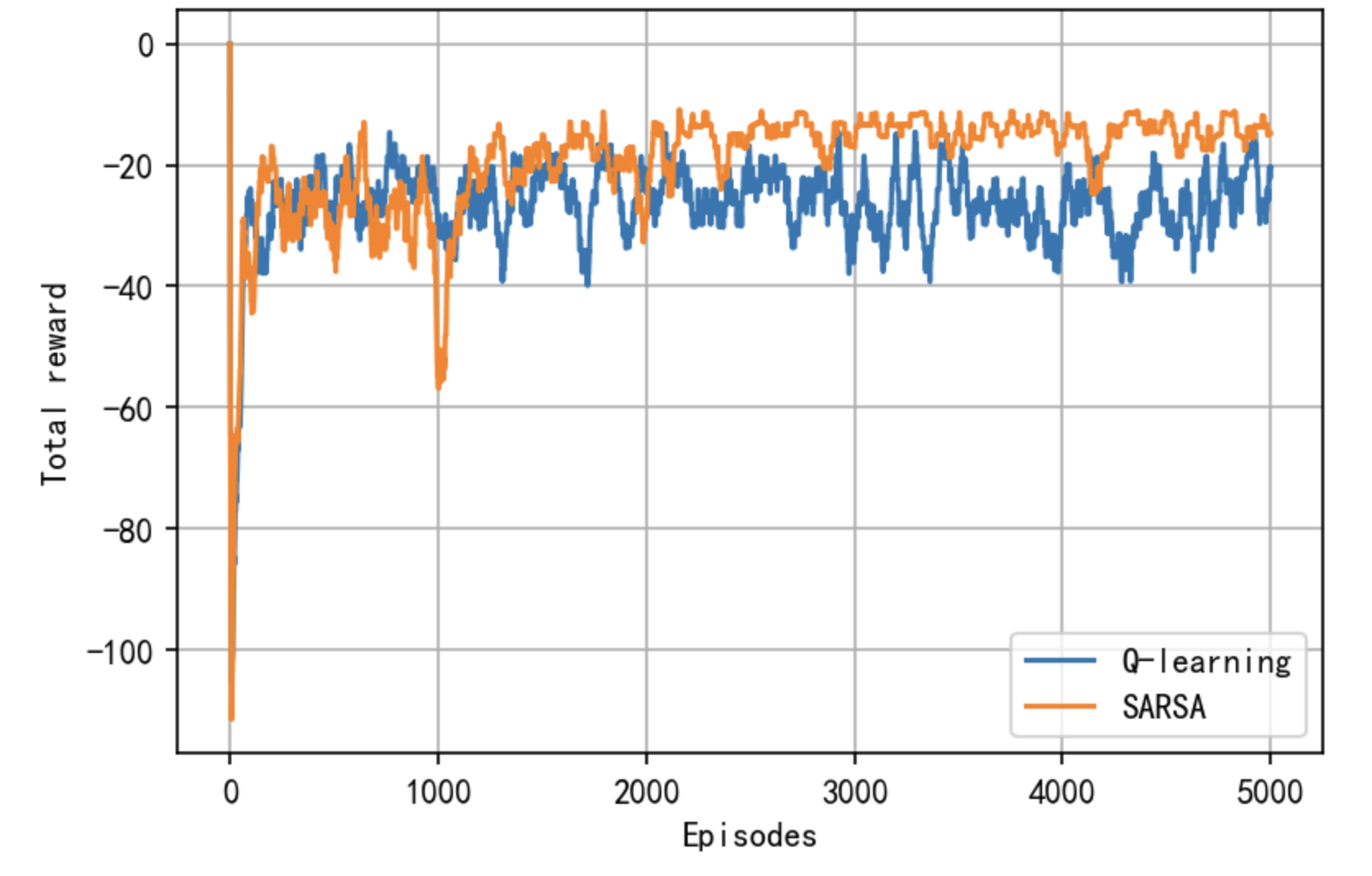
我们将两种算法的每个episode的total rewards画出了,代码如下:
# plot the total reward,Smooth curve by taking the average of total rewards over successive 50 episodes

set_num = 50

total_reward_sarsa_smooth = np.zeros(max_ep)
total_reward_qlearning_smooth = np.zeros(max_ep)

for i in range(0,max_ep):
    if i < set_num:
        total_reward_sarsa_smooth[i] = np.sum(total_reward_sarsa[0:i]) / (i+1)
        total_reward_qlearning_smooth[i] = np.sum(total_reward_qlearning[0:i]) / (i+1)
    else:
        total_reward_sarsa_smooth[i] = np.sum(total_reward_sarsa[i-set_num:i]) / set_num
        total_reward_qlearning_smooth[i] = np.sum(total_reward_qlearning[i-set_num:i]) / set_num


plt.figure(dpi=150)
plt.plot(total_reward_qlearning_smooth,label='Q-learning')
plt.plot(total_reward_sarsa_smooth,label='SARSA')
plt.xlabel('Episodes')
plt.ylabel('Total reward')
plt.legend()
plt.grid(True)
plt.show()
我们观察 Sarsa 和 Q-learning 在训练过程中的回报曲线图,可以发现,随着训练次数增多,在一个episode中 Sarsa 获得的期望回报是高于 Q-learning 的。这是因为在训练过程中智能体采取基于当前 Q ( s , a ) Q(s,a) Q(s,a)函数的 ϵ \epsilon ϵ-贪婪策略来平衡探索与利用,Q-learning 算法由于沿着悬崖边走,会以一定概率探索“掉入悬崖”这一动作,而 Sarsa 相对保守的路线使智能体几乎不可能掉入悬崖,所以SARSA的每个episode的回报更高,但事实上还是Q-learning的策略更优(如果训练完得到Q之后,采取贪婪策略而不是 ϵ \epsilon ϵ-贪婪策略)。
七、总结
本章介绍了无模型的强化学习中的一种非常重要的算法——时序差分算法。时序差分算法的核心思想是用对未来动作选择的价值估计来更新对当前动作选择的价值估计,这是强化学习中的核心思想之一。本章重点讨论了 Sarsa 和 Q-learning 这两个最具有代表性的时序差分算法。当环境是有限状态集合和有限动作集合时,这两个算法非常好用,可以根据任务是否允许在线策略学习来决定使用哪一个算法。
八、参考资料
- Zhao, S… Mathematical Foundations of Reinforcement Learning. Springer Nature Press and Tsinghua University Press.
- Sutton, Richard S., and Andrew G. Barto. Reinforcement learning: An introduction. MIT press, 2018.


 1615
1615

 被折叠的 条评论
为什么被折叠?
被折叠的 条评论
为什么被折叠?
 到【灌水乐园】发言


