Chapter 1 - 8: Temporal-Difference Methods

Chapter 1 - 8: Temporal-Difference Methods

1.8.1 Introduction

  Monte Carlo learning need breaks, it needed the episode to end so that the return could be calculated and then used as estimate for the action values.
  A self-driving car at every turn will be able to estimate if it’s likely to crash, and if necessary, amend its strategy to avoid disaster.
  To emphasize, the Monte Carlo approach would have this car crash every time it wants to learn anything.
  Instead of waiting to update values when the interaction ends, it will amend its predictions at every step, and you’ll be able to use it to solve both continuous and episodic tasks.

1.8.2 Review: MC Control Methods

$$Q(S_t,A_t)\leftarrow Q(S_t,A_t)+\alpha (G_t-Q(S_t,A_t))$$
 where $G_t:={\sum }_{s=t+1}^T{\gamma }^{s-t-1}{R}_s$G is the return at timestep tt, and $Q(S_t,A_t)$ is the entry in the Q-table corresponding to state $S_t$ and action $A_t$.

 The main idea behind this update equation is that $Q(S_t,A_t)$ contains the agent’s estimate for the expected return if the environment is in state $S_t$ and the agent selects action $A_t$. If the return $G_t$ is not equal to $Q(S_t,A_t)$, then we push the value of $Q(S_t,A_t)$ to make it agree slightly more with the return. The magnitude of the change that we make to $Q(S_t,A_t)$ is controlled by the hyperparameter $\alpha >0$.

1.8.3 Quiz: MC Control Methods

1.8.4 TD Control: Sarsa

 Monte Carlo (MC) control methods require us to complete an entire episode of interaction before updating the Q-table. Temporal Difference (TD) methods will instead update the Q-table after every time step.

  We’ll update the Q-Table at the same time as the episode is unfolding.

 In order to use monte carlo method, we sample a complete episode, Then, we look up the current estimate and the Q table, and compare to the return that we actually experienced after visiting the state action pair. We use that new return to make Q table a little more accurate.

 Now, change the update equation to only use a very small time window of information. Instead of using the return as an alternative estimate for updating the Q table. We use the sum of the immediate reward and the discounted value of the next state action pair.

  With the exception of this new update step, it’s identical to what we did in the Monte Carlo case. In particular, we’ll use the epsilon greedy policy to select actions at every time step. The only real difference is what we update the Q table at every time step instead of waitting until the end of the episode, and as long as we specify appropriate values for epsilon, the algorithm is guaranteed to converge to the optimal policy.

Pseudocode

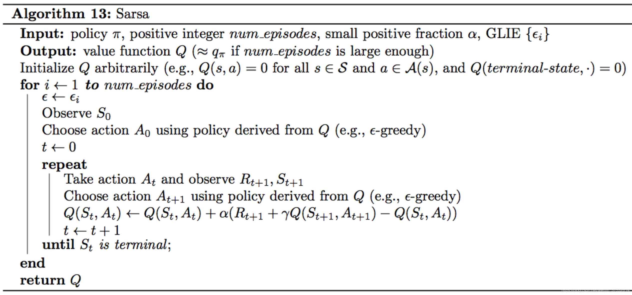
In the algorithm, the number of episodes the agent collects is equal to $num\_episodes$. For every time step $t\ge 0$, the agent:

• takes the action $A_t$ (from the current state $S_t$) that is $ϵ$-greedy with respect to the Q-table,
• receives the reward $R_{t+1}$ and next state $S_{t+1}$,
• chooses the next action $A_{t+1}$ (from the next state $S_{t+1}$) that is $ϵ$-greedy with respect to the Q-table,
• uses the information in the tuple $(S_t,A_t,R_{t+1},S_{t+1},A_{t+1})$ to update the entry $Q(S_t,A_t)$ in the Q-table corresponding to the current state $S_t$ and the action $A_t$.

1.8.5 Quiz: Sarsa

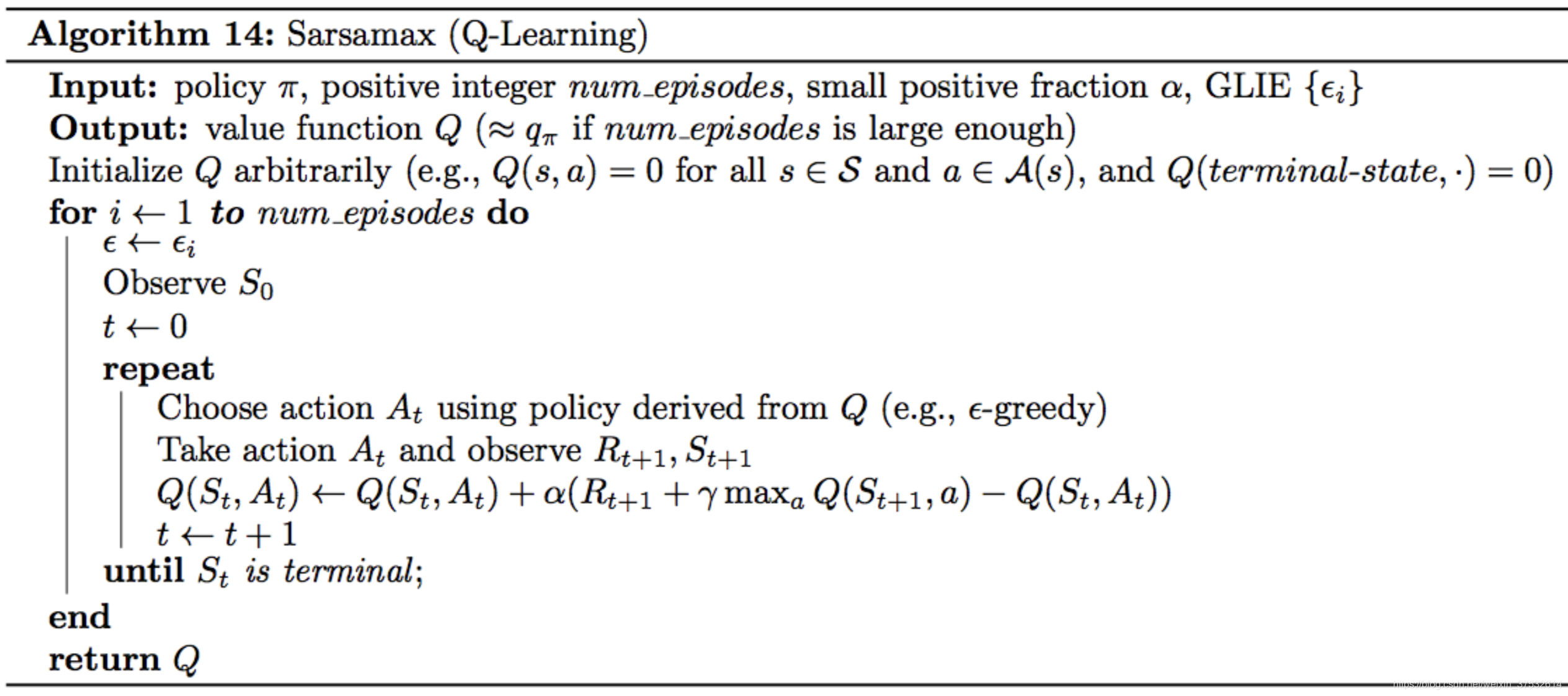
1.8.6 TD Control: Q-Learning

Q-Leaning == Sarsamax

控制问题：通过与环境的交互，获取最优策略的过程

In the Sarsa algorithm, we begin by initializing all action values to zero in constructing the corresponding Epsilon Greedy policy. Then the agent begins interacting with the environment and receives the first state. Next, it uses the policy to choose it’s action.Immediately after if, it receives a reward and next state. Then, the agent again uses the same policy to pick the next action. After choosing that action, it updates the action value corresponding to the previous state action pair, and improves the policy to be epsilon greedy with respect to the most recent estimate of the action values.

We’ll still begin with the same initial values for the action values and the policy. The agent reveives the initial state, the first action is still chosen from the initial policy. But then, after receiving the reward and next state, we’ll update the policy before choosing the next action.
Well, in the sarsa case, our update step was one step later and plugged in action that was selected using the Epsilon Greedy policy. And for every step of the algorithm, if was the case that all of the actions we used for updating the action values, exactly coincide with those that were experienced by the agent. But in general, this does not have to be the case. In particular, consider using the action from the Greedy policy, instead of the Epsilon Greedy policy. This is in fact what Sarsamax of Q-Learning does. We can rewrite the equation to look like this where we rely on the fact that the greedy action corresponding to a state is just the one that maximizes the action values for that state. And so what happens is after we update the action value for time step zero using the greedy action, we then select A1 using Epsilon Greedy policy corresponding to the action values we just updated. And this continues when we received a reward and next state.

In Sarsa, the update step pushes the action values closer to evaluating whatever Epsilon greedy policy is currently being followed by the agent. Sarsamax instead directly attempts to approximate the optimal value function at every time step.

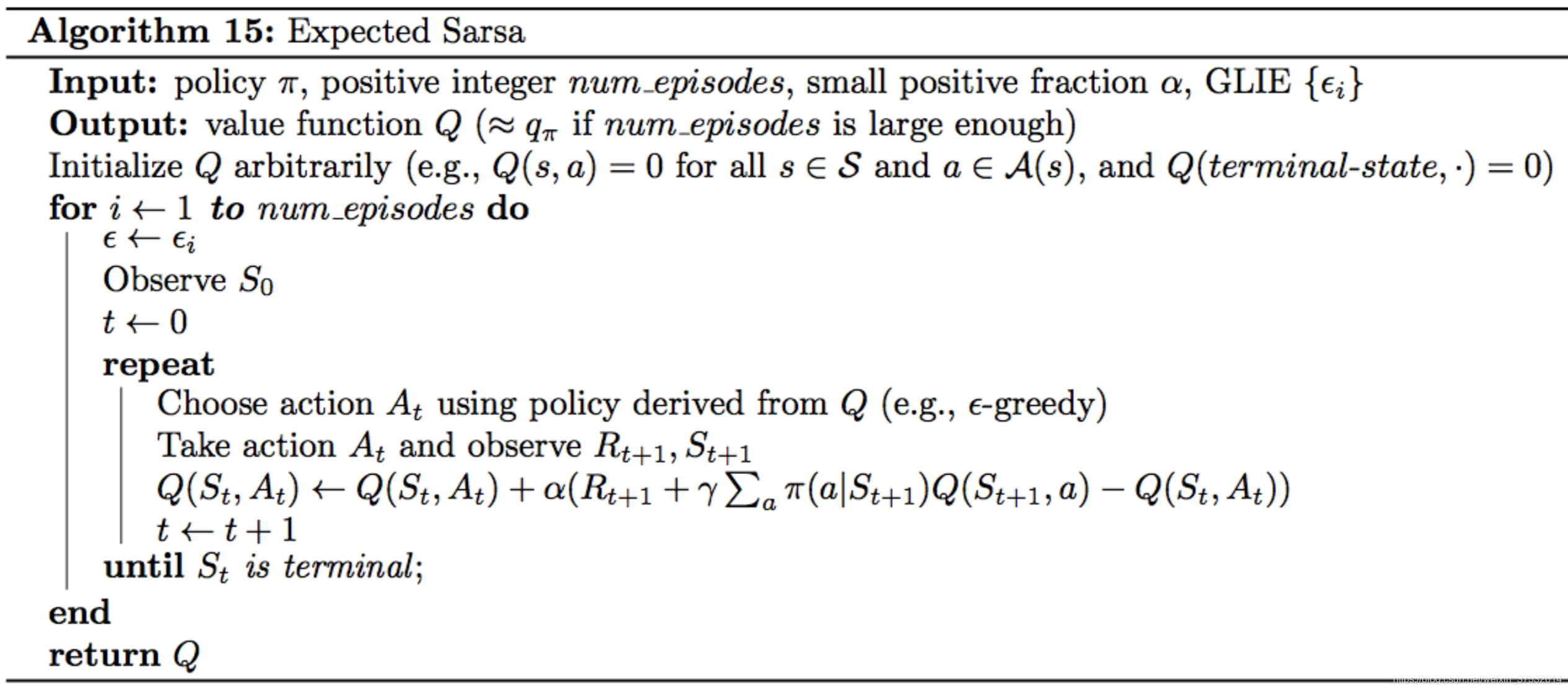
1.8.8 TD Control: Expected Sarsa

It uses the expected value of the next state action pair, where the expectation takes into account the probability that the agent selects each possible action from the next state.

1.8.10 TD Control: Theory and Practice

Greedy in the Limit with Infinite Exploration (GLIE)
 There are many ways to satisfy the GLIE conditions, all of which involve gradually decaying the value of $ϵ$ when constructing $ϵ$-greedy policies.
  In particular, let ${ϵ}_i$ correspond to the $i$-th time step. Then, to satisfy the GLIE conditions, we need only set ${ϵ}_i$ such that:
${ϵ}_i>0$ for all time steps $i$, and ${ϵ}_i$ decays to zero in the limit as the time step $i$i approaches infinity (that is, ${\lim }_{i\to \infty }{ϵ}_i=0)$,

In Theory
 All of the TD control algorithms we have examined (Sarsa, Sarsamax, Expected Sarsa) are guaranteed to converge to the optimal action-value function $q_{\ast }$, as long as the step-size parameter $\alpha$ is sufficiently small, and the GLIE conditions are met.
 Once we have a good estimate for $q_{\ast }$, a corresponding optimal policy ${\pi }_{\ast }$ can then be quickly obtained by setting ${\pi }_{\ast }(s)=\arg {\max }_{a\in \mathcal{A}(s)}{q}_{\ast }(s,a)$ for all $s\in \mathcal{S}$.

In Practice
 In practice, it is common to completely ignore the GLIE conditions and still recover an optimal policy.

Optimism
You have learned that for any TD control method, you must begin by initializing the values in the Q-table. It has been shown that initializing the estimates to large values can improve performance. For instance, if all of the possible rewards that can be received by the agent are negative, then initializing every estimate in the Q-table to zeros is a good technique. In this case, we refer to the initialized Q-table as optimistic, since the action-value estimates are guaranteed to be larger than the true action values.

1.8.11 OpenAI Gym: CliffWalkingEnv

 In order to master the algorithms discussed in this lesson, you will write your own implementations in Python. While your code will be designed to work with any OpenAI Gym environment, you will test your code with the CliffWalking environment.

 In the CliffWalking environment, the agent navigates a 4x12 gridworld.

    """
    This is a simple implementation of the Gridworld Cliff
    reinforcement learning task.
    Adapted from Example 6.6 from Reinforcement Learning: An Introduction
    by Sutton and Barto:
    http://people.inf.elte.hu/lorincz/Files/RL_2006/SuttonBook.pdf

    With inspiration from:
    https://github.com/dennybritz/reinforcement-learning/blob/master/lib/envs/cliff_walking.py
    The board is a 4x12 matrix, with (using Numpy matrix indexing):
        [3, 0] as the start at bottom-left
        [3, 11] as the goal at bottom-right
        [3, 1..10] as the cliff at bottom-center
    Each time step incurs -1 reward, and stepping into the cliff incurs -100 reward 
    and a reset to the start. An episode terminates when the agent reaches the goal.
    """

1.8.14 Workspace

Part 0: Explore CliffWalkingEnv

import sys
import gym
import numpy as np
from collections import defaultdict, deque
import matplotlib.pyplot as plt
%matplotlib inline

import check_test
from plot_utils import plot_values

env = gym.make('CliffWalking-v0')

The agent moves through a 4×12 gridworld, with states numbered as follows:
[[ 0, 1, 2, 3, 4, 5, 6, 7, 8, 9, 10, 11],
[12, 13, 14, 15, 16, 17, 18, 19, 20, 21, 22, 23],
[24, 25, 26, 27, 28, 29, 30, 31, 32, 33, 34, 35],
[36, 37, 38, 39, 40, 41, 42, 43, 44, 45, 46, 47]]
At the start of any episode, state 36 is the initial state. State 47 is the only terminal state, and the cliff corresponds to states 37 through 46.
The agent has 4 potential actions:
UP = 0
RIGHT = 1
DOWN = 2
LEFT = 3

Thus, S+={0,1,…,47}\mathcal{S}^+=\{0, 1, \ldots, 47\}S+={0,1,…,47}, and A={0,1,2,3}\mathcal{A} =\{0, 1, 2, 3\}A={0,1,2,3} . Verify this by running the code cell below.

print(env.action_space)
print(env.observation_space)

 In this mini-project, we will build towards finding the optimal policy for the CliffWalking environment. The optimal state-value function is visualized below. Please take the time now to make sure that you understand why this is the optimal state-value function.

# define the optimal state-value function
V_opt = np.zeros((4,12))
V_opt[0:13][0] = -np.arange(3, 15)[::-1]
V_opt[0:13][1] = -np.arange(3, 15)[::-1] + 1
V_opt[0:13][2] = -np.arange(3, 15)[::-1] + 2
V_opt[3][0] = -13

plot_values(V_opt)

Part 1: TD Control: Sarsa

check_test.py

import unittest 
from IPython.display import Markdown, display
import numpy as np

def printmd(string):
    display(Markdown(string))

V_opt = np.zeros((4,12))
V_opt[0:13][0] = -np.arange(3, 15)[::-1]
V_opt[0:13][1] = -np.arange(3, 15)[::-1] + 1
V_opt[0:13][2] = -np.arange(3, 15)[::-1] + 2
V_opt[3][0] = -13

pol_opt = np.hstack((np.ones(11), 2, 0))

V_true = np.zeros((4,12))
for i in range(3):
    V_true[0:13][i] = -np.arange(3, 15)[::-1] - i
V_true[1][11] = -2
V_true[2][11] = -1
V_true[3][0] = -17

def get_long_path(V):
    return np.array(np.hstack((V[0:13][0], V[1][0], V[1][11], V[2][0], V[2][11], V[3][0], V[3][11])))

def get_optimal_path(policy):
    return np.array(np.hstack((policy[2][:], policy[3][0])))

class Tests(unittest.TestCase):

    def td_prediction_check(self, V):
        to_check = get_long_path(V)
        soln = get_long_path(V_true)
        np.testing.assert_array_almost_equal(soln, to_check)

    def td_control_check(self, policy):
        to_check = get_optimal_path(policy)
        np.testing.assert_equal(pol_opt, to_check)

check = Tests()

def run_check(check_name, func):
    try:
        getattr(check, check_name)(func)
    except check.failureException as e:
        printmd('**<span style="color: red;">PLEASE TRY AGAIN</span>**')
        return
    printmd('**<span style="color: green;">PASSED</span>**')

plot_utils.py

import unittest 
from IPython.display import Markdown, display
import numpy as np

def printmd(string):
    display(Markdown(string))

V_opt = np.zeros((4,12))
V_opt[0:13][0] = -np.arange(3, 15)[::-1]
V_opt[0:13][1] = -np.arange(3, 15)[::-1] + 1
V_opt[0:13][2] = -np.arange(3, 15)[::-1] + 2
V_opt[3][0] = -13

pol_opt = np.hstack((np.ones(11), 2, 0))

V_true = np.zeros((4,12))
for i in range(3):
    V_true[0:13][i] = -np.arange(3, 15)[::-1] - i
V_true[1][11] = -2
V_true[2][11] = -1
V_true[3][0] = -17

def get_long_path(V):
    return np.array(np.hstack((V[0:13][0], V[1][0], V[1][11], V[2][0], V[2][11], V[3][0], V[3][11])))

def get_optimal_path(policy):
    return np.array(np.hstack((policy[2][:], policy[3][0])))

class Tests(unittest.TestCase):

    def td_prediction_check(self, V):
        to_check = get_long_path(V)
        soln = get_long_path(V_true)
        np.testing.assert_array_almost_equal(soln, to_check)

    def td_control_check(self, policy):
        to_check = get_optimal_path(policy)
        np.testing.assert_equal(pol_opt, to_check)

check = Tests()

def run_check(check_name, func):
    try:
        getattr(check, check_name)(func)
    except check.failureException as e:
        printmd('**<span style="color: red;">PLEASE TRY AGAIN</span>**')
        return
    printmd('**<span style="color: green;">PASSED</span>**')

Your algorithm has four arguments:

• env: This is an instance of an OpenAI Gym environment.
• num_episodes: This is the number of episodes that are generated through agent-environment interaction.
• alpha: This is the step-size parameter for the update step.
• gamma: This is the discount rate. It must be a value between 0 and 1, inclusive (default value: 1).

The algorithm returns as output:

• Q: This is a dictionary (of one-dimensional arrays) where Q[s][a] is the estimated action value corresponding to state s and action a.

def update_Q(Qsa, Qsa_next, reward, alpha, gamma):
    """ updates the action-value function estimate using the most recent time step """
    return Qsa + alpha * (reward + gamma * Qsa_next - Qsa)

def epsilon_greedy_probs(env, Q_s, i_episode, eps=False):
    """obtains the action probabilities corresponding to epsilon greedy policy"""
    epsilon = 1.0 / i_episode
    if eps is not None:
        epsilon = eps
    policy_s = np.ones(env.nA) * epsilon / env.nA
    policy_s[np.argmax(Q_s)] = 1- epsilon + (epsilon / env.nA)
    return policy_s

def sarsa(env, num_episodes, alpha, gamma=1.0):
    # initialize action-value function (empty dictionary of arrays)
    Q = defaultdict(lambda: np.zeros(env.nA))
    # initialize performance monitor
    plot_every = 100
    tmp_scores = deque(maxlen=plot_every)
    scores = deque(maxlen=num_episodes)
    
    # loop over episodes
    for i_episode in range(1, num_episodes+1):
        # monitor progress
        if i_episode % plot_every == 0:
            print("\rEpisode {}/{}".format(i_episode, num_episodes), end="")
            sys.stdout.flush()   
        
        ## TODO: complete the function
        # initialize score
        score = 0
        # begin an episode, observe S 
        state = env.reset()
        # get epsilon-greedy action probabilities
        policy_s = epsilon_greedy_probs(env, Q[state], i_episode)
        # pick action
        action = np.random.choice(np.arange(env.nA), p=policy_s)
        # limit number of time steps per episode
        for t_step in np.arange(300):
            # take action A, observe R, S'
            next_state, reward, done, info = env.step(action)
            # add reward to score
            score += reward
            if not done:
                # get epsilon-greedy action probabilities
                policy_s = epsilon_greedy_probs(env, Q[state], i_episode)
                # pick action
                next_action = np.random.choice(np.arange(env.nA), p=policy_s)
                Q[state][action] = update_Q(Q[state][action], Q[next_state][next_action], reward, alpha, gamma)
                state = next_state
                action = next_action
            if done:
                Q[state][action] = update_Q(Q[state][action], 0, reward, alpha, gamma)
                # append score
                tmp_scores.append(score)
                break
        if (i_episode % plot_every ==0):
            scores.append(np.mean(tmp_scores))
    # plot performance
    plt.plot(np.linspace(0, num_episodes, len(scores), endpoint=False),np.asarray(scores))
    plt.xlabel('Episode Number')
    plt.ylabel('Average Reward (Over Next %d Episodes)' % plot_every)
    plt.show()
    # print best 100-episode performance
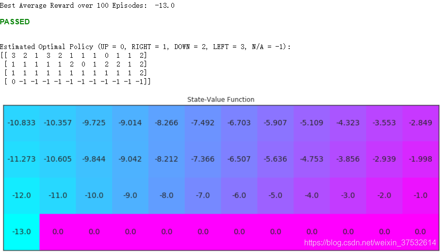
    print(('Best Average Reward over %d Episodes: ' % plot_every), np.max(scores))
    return Q

# obtain the estimated optimal policy and corresponding action-value function
Q_sarsa = sarsa(env, 5000, .01)

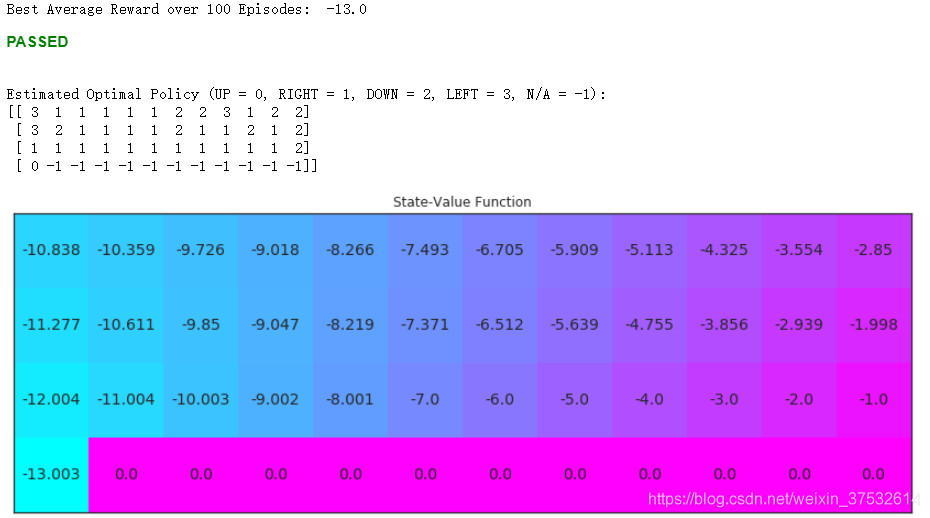
# print the estimated optimal policy
policy_sarsa = np.array([np.argmax(Q_sarsa[key]) if key in Q_sarsa else -1 for key in np.arange(48)]).reshape(4,12)
check_test.run_check('td_control_check', policy_sarsa)
print("\nEstimated Optimal Policy (UP = 0, RIGHT = 1, DOWN = 2, LEFT = 3, N/A = -1):")
print(policy_sarsa)

# plot the estimated optimal state-value function
V_sarsa = ([np.max(Q_sarsa[key]) if key in Q_sarsa else 0 for key in np.arange(48)])
plot_values(V_sarsa)

Part 2: TD Control: Q-learning

Your algorithm has four arguments:

• env: This is an instance of an OpenAI Gym environment.
• num_episodes: This is the number of episodes that are generated through agent-environment interaction.
• alpha: This is the step-size parameter for the update step.
• gamma: This is the discount rate. It must be a value between 0 and 1, inclusive (default value: 1).

The algorithm returns as output:

• Q: This is a dictionary (of one-dimensional arrays) where Q[s][a] is the estimated action value corresponding to state s and action a.

def q_learning(env, num_episodes, alpha, gamma=1.0):
    # initialize empty dictionary of arrays
    Q = defaultdict(lambda: np.zeros(env.nA))
    # initialize performance monitor
    plot_every = 100
    tmp_scores = deque(maxlen=plot_every)
    scores = deque(maxlen=num_episodes)
    # loop over episodes
    for i_episode in range(1, num_episodes+1):
        # monitor progress
        if i_episode % 100 == 0:
            print("\rEpisode {}/{}".format(i_episode, num_episodes), end="")
            sys.stdout.flush()
        
        ## TODO: complete the function
        # initialize score
        score = 0
        # begin an episode, observe S 
        state = env.reset()
        
        # limit number of time steps per episode
        while True:
            # get epsilon-greedy action probabilities
            policy_s = epsilon_greedy_probs(env, Q[state], i_episode)
            # pick action
            action = np.random.choice(np.arange(env.nA), p=policy_s)
            # take action A, observe R, S'
            next_state, reward, done, info = env.step(action)
            # add reward to score
            score += reward
            # print(score)
            if not done:
                Q[state][action] = update_Q(Q[state][action], np.max(Q[next_state]), reward, alpha, gamma)
                state = next_state
            if done:
                Q[state][action] = update_Q(Q[state][action], 0, reward, alpha, gamma)
                # append score
                tmp_scores.append(score)
                break
        if (i_episode % plot_every ==0):
            #print(i_episode)
            #print(tmp_scores)
            #print(np.sum(tmp_scores))
            #print(np.mean(tmp_scores))
            scores.append(np.mean(tmp_scores))
    # plot performance
    # print(np.asarray(scores))
    plt.plot(np.linspace(0, num_episodes, len(scores), endpoint=False),np.asarray(scores))
    plt.xlabel('Episode Number')
    plt.ylabel('Average Reward (Over Next %d Episodes)' % plot_every)
    plt.grid()
    plt.show()
    # print best 100-episode performance
    print(('Best Average Reward over %d Episodes: ' % plot_every), np.max(scores))
    return Q

# obtain the estimated optimal policy and corresponding action-value function
Q_sarsamax = q_learning(env, 5000, .01)

# print the estimated optimal policy
policy_sarsamax = np.array([np.argmax(Q_sarsamax[key]) if key in Q_sarsamax else -1 for key in np.arange(48)]).reshape((4,12))
check_test.run_check('td_control_check', policy_sarsamax)
print("\nEstimated Optimal Policy (UP = 0, RIGHT = 1, DOWN = 2, LEFT = 3, N/A = -1):")
print(policy_sarsamax)

# plot the estimated optimal state-value function
plot_values([np.max(Q_sarsamax[key]) if key in Q_sarsamax else 0 for key in np.arange(48)])

Part 3: TD Control: Expected Sarsa

In this section, you will write your own implementation of the Expected Sarsa control algorithm.

Your algorithm has four arguments:

• env: This is an instance of an OpenAI Gym environment.
• num_episodes: This is the number of episodes that are generated through agent-environment interaction.
• alpha: This is the step-size parameter for the update step.
• gamma: This is the discount rate. It must be a value between 0 and 1, inclusive (default value: 1).

The algorithm returns as output:

• Q: This is a dictionary (of one-dimensional arrays) where Q[s][a] is the estimated action value corresponding to state s and action a.

1.8.15 Analyzing Performance

Similarities
 All of the TD control methods we have examined (Sarsa, Sarsamax, Expected Sarsa) converge to the optimal action-value function $q_{\ast }$ (and so yield the optimal policy ${\pi }_{\ast }$) if:

1. the value of $ϵ$ decays in accordance with the GLIE conditions, and
2. the step-size parameter $\alpha$ is sufficiently small.

Differences
The differences between these algorithms are summarized below:
On-policy: 无论是根据策略选动作，还是更新Q表的时候使用的策略，都是$ϵ$-贪婪策略
Off-policy:选取动作的时候使用的是$ϵ$-贪婪策略，但是更新Q表的时候使用的是贪婪策略

• Sarsa and Expected Sarsa are both on-policy TD control algorithms. In this case, the same (\epsilonϵ-greedy) policy that is evaluated and improved is also used to select actions.
• Sarsamax is an off-policy method, where the (greedy) policy that is evaluated and improved is different from the (\epsilonϵ-greedy) policy that is used to select actions.
• On-policy TD control methods (like Expected Sarsa and Sarsa) have better online performance than off-policy TD control methods (like Sarsamax).
• Expected Sarsa generally achieves better performance than Sarsa.

1.8.17 Summary

Temporal-Difference Methods

• Whereas Monte Carlo (MC) prediction methods must wait until the end of an episode to update the value function estimate, temporal-difference (TD) methods update the value function after every time step.

TD Control

• Sarsa(0) (or Sarsa) is an on-policy TD control method. It is guaranteed to converge to the optimal action-value function $q_{\ast }$, as long as the step-size parameter $\alpha$ is sufficiently small and $ϵ$ is chosen to satisfy the Greedy in the Limit with Infinite Exploration (GLIE) conditions.
• Sarsamax (or Q-Learning) is an off-policy TD control method. It is guaranteed to converge to the optimal action value function $q_{\ast }$, under the same conditions that guarantee convergence of the Sarsa control algorithm.
• Expected Sarsa is an on-policy TD control method. It is guaranteed to converge to the optimal action value function $q_{\ast }$, under the same conditions that guarantee convergence of Sarsa and Sarsamax.

Analyzing Performance

• On-policy TD control methods (like Expected Sarsa and Sarsa) have better online performance than off-policy TD control methods (like Q-learning).
• Expected Sarsa generally achieves better performance than Sarsa.