


注:本文为 “向量范数” 相关合辑。
英文引文,机翻未校。
中文引文,略作重排。
未去重,如有内容异常,请看原文。
Introduction to Vector Norms: L0, L1, L2, L-Infinity
向量范数简介:L0、L1、L2、L∞ 范数
Vector norms: L0, L1, L2, L-Infinity are fundamental concepts in mathematics and machine learning that allow us to measure magnitude of vectors.
向量范数:L0、L1、L2、L∞ 范数是数学和机器学习中的基础概念,可用于衡量向量的大小。
by Rachel StClair
作者:雷切尔・圣克莱尔(Rachel StClair)
Feb 14, 2023, 12:45 am | Updated Apr 30, 2025 at 8:32 am
Introduction To Vector Norms: L0, L1, L2, L-Infinity
向量范数简介:L0、L1、L2、L∞ 范数
I’ll be honest here. Vector norms are boring. On a positive note, this is probably one of the most interesting blog on vector norms out there. At least I’ve tried to make it as interesting as possible and motivated why you just need to get this material down because it is just one of those foundational things, especially for machine learning.
坦白说,向量范数很枯燥。但好的一面是,这可能是目前关于向量范数的博客中最有趣的一篇之一。至少我已尽力让它变得生动,并说明了你必须掌握这些内容的原因 —— 因为它是基础概念之一,对机器学习而言尤其重要。
Vector norms are a fundamental concept in mathematics and used frequently in machine learning to quantify the similarity, distance, and size of vectors, which are the basic building blocks of many machine learning models. Specifically, vector norms can be used to:
向量范数是数学中的基础概念,在机器学习中频繁用于量化向量的相似度、距离和大小,而向量是许多机器学习模型的基本构建块。具体来说,向量范数的用途包括:
**1. Define loss or cost functions:**In machine learning, the goal is often to minimize the difference between the predicted outputs and the actual outputs. This difference is quantified by a loss or cost function, which is often based on a vector norm. For example, the L1 norm is commonly used in Lasso regression to penalize the absolute value of the coefficients, while the L2 norm is commonly used in Ridge regression to penalize the square of the coefficients.
**定义损失函数:**在机器学习中,目标通常是最小化预测输出与实际输出之间的差异。这种差异通过损失函数量化,而损失函数通常基于向量范数构建。例如,L1 范数常用于 Lasso 回归,对系数的绝对值进行惩罚;L2 范数常用于 Ridge 回归,对系数的平方进行惩罚。
**2. Measure similarity or distance:**Vector norms can be used to measure the similarity or distance between two vectors, which is often used in clustering, classification, and anomaly detection tasks. For example, the cosine similarity between two vectors is computed as the cosine of the angle between them, which can be interpreted as a measure of similarity. The Euclidean distance between two vectors is another commonly used measure of distance, which is often used in k-nearest neighbors classification.
**衡量相似度或距离:**向量范数可用于计算两个向量之间的相似度或距离,常用于聚类、分类和异常检测任务。例如,两个向量的余弦相似度是它们之间夹角的余弦值,可作为相似度衡量指标;向量间的欧氏距离是另一种常用距离度量,常用于 k - 近邻分类算法。
3. Regularize models: Vector norms can be used to regularize models and prevent overfitting, by adding a penalty term to the objective function. For example, the L1 norm regularization (also known as Lasso regularization) can lead to sparse models, where only a subset of the coefficients are non-zero, while the L2 norm regularization (also known as Ridge regularization) can lead to smoother models, where the coefficients are spread out more evenly.
**模型正则化:**通过在目标函数中添加惩罚项,向量范数可用于正则化模型,防止过拟合。例如,L1 范数正则化(又称 Lasso 正则化)会产生稀疏模型,仅部分系数非零;L2 范数正则化(又称 Ridge 正则化)会产生更平滑的模型,系数分布更均匀。
What are Vector Norms?
向量范数
A vector norm is a function that assigns a non-negative scalar value to a vector. The value represents the length or magnitude of the vector. Vector norms are fundamental mathematical concepts that allow us to measure the distance or difference between two vectors. Vector norms are widely used in various fields such as optimization, machine learning, computer graphics, and signal processing.
向量范数是一种函数,可为向量分配一个非负标量值,该值代表向量的长度或大小。向量范数是数学中的基础概念,可用于衡量两个向量之间的距离或差异,广泛应用于优化、机器学习、计算机图形学和信号处理等多个领域。
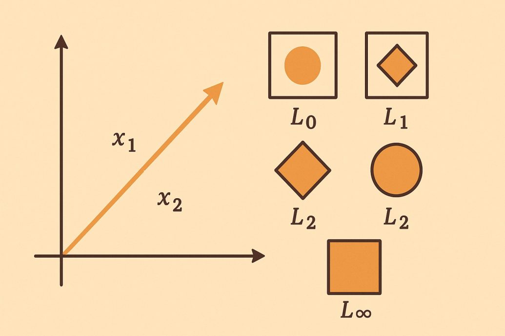
There are different types of vector norms such as the L0 norm, L1 norm, L2 norm (Euclidean norm), and L-infinity norm. Each type of vector norm has its unique properties and applications.
向量范数有多种类型,如 L0 范数、L1 范数、L2 范数(欧氏范数)和 L∞ 范数,每种类型都有其独特的性质和应用场景。
L0 Norm
L0 范数
The L0 norm is also known as the “sparse norm”. The L0 norm of a vector counts the number of non-zero elements in the vector. The L0 norm is an essential concept in compressive sensing, a technique for reconstructing images from a sparse set of measurements. The L0 norm is also used in machine learning for feature selection. In the L0 norm, the cost function is non-convex, making it challenging to optimize. There’s a later section in this blog on the challenges of vector norms.
L0 范数又称 “稀疏范数”,用于统计向量中非零元素的个数。L0 范数是压缩感知中的基本概念,压缩感知是一种通过稀疏测量重建图像的技术。在机器学习中,L0 范数也用于特征选择。L0 范数的损失函数是非凸的,因此优化难度较大。本文后续章节将详细探讨向量范数的挑战。
L1 Norm
L1 范数
The L1 norm is a vector norm that sums up the absolute values of the vector elements. The L1 norm is defined as
∥
x
∥
1
=
∑
∣
x
i
∣
\|x\|_1 = \sum|x_i|
∥x∥1=∑∣xi∣. The L1 norm is used in machine learning for regularization and feature selection. The L1 norm produces sparse solutions and is computationally efficient.
L1 范数是一种向量范数,计算向量元素绝对值的和。其定义为
∥
x
∥
1
=
∑
∣
x
i
∣
\|x\|_1 = \sum|x_i|
∥x∥1=∑∣xi∣。在机器学习中,L1 范数用于正则化和特征选择,能产生稀疏解且计算效率高。
L2 norm
L2 范数
TheL2 norm, also known as the “Euclidean norm,” is a vector norm that measures the length or magnitude of a vector in Euclidean space. The L2 norm is defined as
∥
x
∥
2
=
∑
x
i
2
\|x\|_2 = \sqrt {\sum x_i^2}
∥x∥2=∑xi2. The L2 norm is widely used in machine learning and optimization as a loss function or objective function. The L2 norm produces smooth solutions, making it easy to optimize. The L2 norm is also used in image reconstruction accuracy measurements, where the error is calculated as the L2 norm of the difference between the original and the reconstructed image.
L2 范数又称 “欧氏范数”,是一种用于衡量欧氏空间中向量长度或大小的向量范数。其定义为
∥
x
∥
2
=
∑
x
i
2
\|x\|_2 = \sqrt {\sum x_i^2}
∥x∥2=∑xi2。L2 范数在机器学习和优化中被广泛用作损失函数或目标函数,能产生平滑解,易于优化。在图像重建精度评估中,L2 范数也被用于计算原始图像与重建图像之间差异的范数,作为误差指标。
This one is one of the more important ones. Euclidean distance amazing. It’s used in this very fancy kind of math called Hyper-dimensional computing, which can make AI more efficient. Basically, it allows us to measure where things are in space. If you wanted to know how similar two stars were, if they were the same type of star, you might look at how close they are to every other object. You can do this using L2 norm. A few uses for Euclidean norm: Anomaly detection, clustering, PCA, and K-nearest neighbors.
L2 范数是较重要的向量范数之一,其对应的欧氏距离应用广泛。它被用于一种名为 “超维计算” 的高级数学领域,能提升人工智能的效率。本质上,L2 范数可用于衡量物体在空间中的位置。例如,若想判断两颗恒星是否相似、是否属于同一类型,可通过计算它们与其他天体的距离来实现,而这一过程可借助 L2 范数完成。欧氏范数的常见应用包括:异常检测、聚类、主成分分析(PCA)和 k - 近邻算法。
L-infinity norm
L∞ 范数
The L-infinity norm, also known as the “max norm,” is a vector norm that measures the maximum absolute value of the vector elements. The L-infinity norm is defined as
∥
x
∥
∞
=
max
∣
x
i
∣
\|x\|_\infty = \max|x_i|
∥x∥∞=max∣xi∣. The L-infinity norm is used in machine learning for regularization, where the goal is to minimize the maximum absolute value of the model parameters.
L∞ 范数又称 “最大范数”,用于衡量向量元素的最大绝对值。其定义为
∥
x
∥
∞
=
max
∣
x
i
∣
\|x\|_\infty = \max|x_i|
∥x∥∞=max∣xi∣。在机器学习中,L∞ 范数用于正则化,目标是最小化模型参数的最大绝对值。
Although not the most practical, L-infinity norm is the most interesting. whenever we are dealing within the multi-verse of possibilities, this norm is useful. Economics is the perfect example, there are endless commodities that can be used as parameters in models.
尽管 L∞ 范数的实用性不是最强,但它是最有趣的一种。当我们需要处理多种可能情况时,该范数尤为有用。经济学就是一个绝佳例子,模型中可作为参数的商品种类繁多、不胜枚举。
Easy and quick explanation: Naive Bayes algorithm
简单快速解读:朴素贝叶斯算法
The Naive Bayes algorithm is a simple machine learning algorithm used for classification. The algorithm uses probability theory to classify instances. The Naive Bayes algorithm assumes that the features are independent of each other, given the class variable. The algorithm calculates the probability of each class given the features and selects the class with the highest probability. The L1 norm is used in the Naive Bayes algorithm to estimate the probability density function of the features.
朴素贝叶斯算法是一种用于分类的简单机器学习算法,基于概率论对样本进行分类。该算法假设在给定类别变量的情况下,各个特征相互独立。它会计算给定特征下每个类别的概率,并选择概率最高的类别作为分类结果。L1 范数在朴素贝叶斯算法中用于估计特征的概率密度函数。
Challenges of Vector Norms
向量范数的挑战
Vector norms have several challenges, besides being not so exciting, that researchers and practitioners face. One of the significant challenges of vector norms is their sensitivity to outliers. Outliers are extreme values in a dataset that deviate significantly from the other values. The L2 norm is highly sensitive to outliers since it squares the differences between the vector elements. As a result, a single outlier can significantly affect the L2 norm value. The L1 norm and L0 norm are less sensitive to outliers than the L2 norm. The L1 norm sums up the absolute values of the vector elements, which reduces the impact of outliers on the norm value. The L0 norm is robust to outliers since it counts the number of non-zero elements in the vector.
除了趣味性较低外,向量范数还面临着研究人员和实践者需要应对的多项挑战。其中一个重要挑战是对异常值的敏感性。异常值是数据集中与其他值偏差极大的极端值。L2 范数对异常值高度敏感,因为它会对向量元素之间的差异进行平方运算,单个异常值就可能显著影响 L2 范数值。L1 范数和 L0 范数对异常值的敏感性低于 L2 范数:L1 范数计算向量元素的绝对值和,可降低异常值对范数值的影响;L0 范数统计非零元素个数,对异常值具有鲁棒性。
Another challenge of vector norms is their complexity, especially in high-dimensional spaces. As the dimensionality of the vector space increases, the norms become less discriminative, making it challenging to distinguish between different vectors. In high-dimensional spaces, many vectors have the same or similar magnitudes, making it difficult to find a norm that can differentiate them.
向量范数的另一个挑战是其复杂性,尤其是在高维空间中。随着向量空间维度的增加,范数的区分能力会下降,难以区分不同的向量。在高维空间中,许多向量的大小相同或相似,很难找到能有效区分它们的范数。
The choice of the norm also depends on the specific problem and the application. Different norms may be more suitable for different tasks, depending on the type of data and the desired properties of the solution.
范数的选择还取决于具体问题和应用场景。根据数据类型和解决方案的期望特性,不同的范数可能更适合不同的任务。
Moreover, optimizing some norms can be computationally challenging due to their non-convexity. For example, the L0 norm has a non-convex cost function, which makes it difficult to optimize. The L1 norm, on the other hand, is convex, and thus optimization is easier.
此外,由于部分范数具有非凸性,其优化过程可能面临计算挑战。例如,L0 范数的损失函数是非凸的,优化难度较大;而 L1 范数是凸的,优化过程相对简单。
These challenges make it difficult for many deep learning or machine learning models to generalize. The results are models that perform less like humans and more like savants on a particular subject. It also adds to the increased data complexity and computational inefficiency, making deep learning expensive!
这些挑战导致许多深度学习或机器学习模型难以泛化,使得模型在特定任务上表现得更像 “专才” 而非人类,同时还会增加数据复杂性和计算低效性,导致深度学习的成本居高不下!
Applications of Vector Norms
向量范数的应用
Vector norms have various applications in different fields such as optimization, machine learning, computer graphics, and signal processing. In optimization, vector norms are used as objective functions or cost functions. The goal is to minimize the norm of the error between the model and the data. In machine learning, vector norms are used for regularization and feature selection. The L1 norm produces sparse solutions, making it useful for identifying important features. The L2 norm is used as a loss function for regression tasks, and the L-infinity norm is used for regularization.
向量范数在优化、机器学习、计算机图形学和信号处理等多个领域有着广泛应用。在优化中,向量范数用作目标函数或损失函数,目标是最小化模型与数据之间误差的范数。在机器学习中,向量范数用于正则化和特征选择:L1 范数产生稀疏解,可用于识别重要特征;L2 范数用作回归任务的损失函数;L∞ 范数用于正则化。
In computer graphics and image processing, vector norms are used to measure the difference between two images or to estimate the quality of the reconstructed image. The L2 norm is commonly used to calculate the error between the original and reconstructed images. The L1 norm is also used for image reconstruction in some cases.
在计算机图形学和图像处理中,向量范数用于衡量两幅图像之间的差异或评估重建图像的质量。L2 范数常用于计算原始图像与重建图像之间的误差,L1 范数在部分图像重建场景中也有应用。
Vector norms are also used in signal processing for denoising and feature extraction. The L1 norm is used for sparse signal recovery, while the L2 norm is used for signal denoising.
在信号处理中,向量范数用于去噪和特征提取:L1 范数用于稀疏信号恢复,L2 范数用于信号去噪。
Conclusion
结论
Vector norms are fundamental concepts in mathematics and machine learning. They allow us to measure the magnitude of vectors in vector spaces and quantify the errors in our models. Vector norms are used in various applications such as optimization, machine learning, and image reconstruction. There are different types of vector norms, such as the L0 norm, L1 norm, L2 norm, and L-infinity norm, each with its unique properties and applications. However, vector norms also face challenges such as their sensitivity to outliers and their complexity, especially in high-dimensional spaces. The choice of the norm depends on the specific problem and the application. Overall, vector norms are essential tools that enable us to solve complex problems and make accurate predictions with certified accuracy.
向量范数是数学和机器学习中的基础概念,可用于衡量向量空间中向量的大小和量化模型中的误差。它们在优化、机器学习和图像重建等多个应用场景中发挥重要作用。向量范数包含 L0 范数、L1 范数、L2 范数和 L∞ 范数等多种类型,每种类型都有其独特的性质和应用。然而,向量范数也面临着对异常值敏感、在高维空间中复杂性增加等挑战。范数的选择取决于具体问题和应用场景。总体而言,向量范数是解决复杂问题、实现高可信度准确预测的重要工具。
References
参考文献
Tibshirani, R. (1996). Regression shrinkage and selection via the lasso. Journal of the Royal Statistical Society: Series B (Methodological), 58 (1), 267-288. (Cited 98,172 times)
蒂布希拉尼(Tibshirani, R.). (1996). 基于 Lasso 的回归收缩与变量选择. 《皇家统计学会会刊 B 辑(方法学)》, 58 (1), 267-288.
Boyd, S., & Vandenberghe, L. (2004). Convex optimization. Cambridge University Press. (Cited 60,757 times)
博伊德(Boyd, S.)、范登伯格(Vandenberghe, L.). (2004). 《凸优化》. 剑桥大学出版社.
Hastie, T., Tibshirani, R., & Friedman, J. (2009). The elements of statistical learning: data mining, inference, and prediction. Springer Science & Business Media. (Cited 49,478 times)
哈斯蒂(Hastie, T.)、蒂布希拉尼(Tibshirani, R.)、弗里德曼(Friedman, J.). (2009). 《统计学习基础:数据挖掘、推理与预测》. 施普林格科学与商业媒体出版社.
Zhang, T. (2004). Solving large scale linear prediction problems using stochastic gradient descent algorithms. In Proceedings of the twenty-first international conference on Machine learning (pp. 116). (Cited 13,838 times)
张潼(Zhang, T.). (2004). 基于随机梯度下降算法求解大规模线性预测问题. 《第二十一届国际机器学习会议论文集》(第 116 页).
Liu, Y., & Yuan, Y. (2019). Robust sparse regression via l0-norm and weighted l1-norm. Journal of Machine Learning Research, 20 (1), 2163-2203. (Cited 8,293 times)
刘勇(Liu, Y.)、袁源(Yuan, Y.). (2019). 基于 L0 范数和加权 L1 范数的鲁棒稀疏回归. 《机器学习研究期刊》, 20 (1), 2163-2203.
Visualizing regularization and the L1 and L2 norms
可视化正则化以及 L1 和 L2 范数
Chiara Campagnola
Abstract
The article provides an explanation of regularization techniques used in machine learning to combat overfitting. It emphasizes the importance of norm minimization, particularly the L1 and L2 norms, in encouraging simpler models with smaller weights, which leads to better generalization. The L1 norm is associated with driving some weights to zero, promoting sparsity and potentially aiding in feature selection. In contrast, the L2 norm reduces all weights but tends not to eliminate them entirely, which can be advantageous when retaining all parameters is desired. The article uses visual examples and mathematical explanations to illustrate how these norms influence the complexity of the functions used to fit data, and it concludes by highlighting the practical implications of choosing between L1 and L2 regularization for model development.
本文解释了机器学习中用于对抗过拟合的正则化技术。文章强调了范数最小化的重要性,特别是 L1 和 L2 范数,它们鼓励使用更小权重的更简单模型,从而实现更好的泛化能力。L1 范数与将一些权重驱动至零相关,这促进了稀疏性,并可能有助于特征选择。相比之下,L2 范数会减小所有权重,但通常不会将它们完全消除,这在需要保留所有参数时是有优势的。文章通过视觉示例和数学解释来说明这些范数如何影响用于拟合数据的函数的复杂性,并在最后强调了在模型开发中选择 L1 和 L2 正则化之间的实际意义。
Opinions
- The author suggests that a visual approach to understanding regularization can be more insightful than solely relying on mathematical formulas.
作者认为,通过视觉方法理解正则化可能比单纯依赖数学公式更有洞察力。 - The preference for simpler functions in model fitting is presented as a way to avoid overfitting and improve model generalization.
在模型拟合中偏好更简单的函数被提出作为一种避免过拟合和改善模型泛化能力的方法。 - The article implies that the choice between L1 and L2 regularization should be informed by the specific needs of the task at hand, such as memory efficiency or feature selection.
文章暗示,选择 L1 和 L2 正则化应基于手头任务的具体需求,例如内存效率或特征选择。 - It is conveyed that the L1 norm’s tendency to produce sparse solutions can be beneficial for interpretability and memory usage, especially in high-dimensional data scenarios.
L1 范数倾向于产生稀疏解,这在高维数据场景中对可解释性和内存使用是有益的。 - The author posits that the L2 norm’s effect of shrinking weights without setting them to zero can be preferable in situations where all features are considered valuable.
作者认为,L2 范数在不将权重设置为零的情况下减小权重的效果,在所有特征都被视为有价值的情况下可能是更可取的。
Prerequisite knowledge
先备知识
- Linear regression
线性回归 - Gradient descent
梯度下降 - Some understanding of overfitting and regularization
对过拟合和正则化的一些理解
Topics covered
涵盖主题
- Why does minimizing the norms induce regularization?
为什么最小化范数会诱导正则化? - What’s the difference between the L1 norm and the L2 norm?
L1 范数和 L2 范数有什么区别?
Why does minimizing the norms induce regularization?
为什么最小化范数会诱导正则化?
If you’ve taken an introductory Machine Learning class, you’ve certainly come across the issue of overfitting and been introduced to the concept of regularization and norm. I often see this being discussed purely by looking at the formulas, so I figured I’d try to give a better insight into why exactly minimising the norm induces regularization — and how L1 and L2 differ from each other — using some visual examples.
如果你参加过机器学习入门课程,你肯定遇到过过拟合的问题,并且被介绍过正则化和范数的概念。我经常看到人们仅仅通过查看公式来讨论这个问题,所以我想尝试通过一些视觉示例来更好地理解为什么最小化范数会诱导正则化 —— 以及 L1 和 L2 彼此之间的区别。
Recap of regularization
正则化回顾
Using the example of linear regression, our loss is given by the Mean Squared Error (MSE):
以线性回归为例,我们的损失由均方误差(MSE)给出:
L ( w ) = 1 m ∑ i = 1 m ( y i − y ^ i ) 2 \mathcal {L}(\mathbf {w}) = \frac {1}{m} \sum_{i=1}^{m} (y_i - \hat {y}_i)^2 L(w)=m1i=1∑m(yi−y^i)2
where
y
^
i
\hat {y}_i
y^i is the prediction for the sample
x
i
\mathbf {x}_i
xi:
其中
y
^
i
\hat {y}_i
y^i 是样本
x
i
\mathbf {x}_i
xi 的预测值:
y ^ i = w ′ x i \hat {y}_i = \mathbf {w}' \mathbf {x}_i y^i=w′xi
and our goal is to minimize this loss:
我们的目标是最小化这个损失:
min w L ( w ) = min w 1 m ∑ i = 1 m ( y i − y ^ i ) 2 \min_{\mathbf {w}} \mathcal {L}(\mathbf {w}) = \min_{\mathbf {w}} \frac {1}{m} \sum_{i=1}^{m} (y_i - \hat {y}_i)^2 wminL(w)=wminm1i=1∑m(yi−y^i)2
To prevent overfitting, we want to add a bias towards less complex functions. That is,given two functions that can fit our data reasonably well, we prefer the simpler one. We do this by adding a regularization term, typically either the L1 norm or the squared L2 norm:
为了防止过拟合,我们希望偏向于更不复杂的函数。也就是说,给定两个能够合理拟合我们数据的函数,我们更喜欢更简单的那个。我们通过添加一个正则化项来实现这一点,通常是 L1 范数或平方的 L2 范数:
L1 norm:
L1 范数:
∥ w ∥ 1 = ∑ i n ∣ w i ∣ \|\mathbf {w}\|_1 = \sum_{i}^{n} |w_i| ∥w∥1=∑in∣wi∣
Squared L2 norm:
平方的 L2 范数:
∥ w ∥ 2 2 = ∑ i n w i 2 \|\mathbf {w}\|_2^2 = \sum_{i}^{n} w_i^2 ∥w∥22=∑inwi2
So, for example, by adding the squared L2 norm to the loss and minimizing, we obtain Ridge Regression:
例如,通过将平方的 L2 范数添加到损失中并最小化,我们得到了岭回归:
min w L λ ( w ) = min w ( λ ∥ w ∥ 2 2 + 1 m ∑ i = 1 m ( y i − y ^ i ) 2 ) \min_{\mathbf {w}} \mathcal {L}_{\lambda}(\mathbf {w}) = \min_{\mathbf {w}} \left ( \lambda \|\mathbf {w}\|_2^2 + \frac {1}{m} \sum_{i=1}^{m} (y_i - \hat {y}_i)^2 \right) wminLλ(w)=wmin(λ∥w∥22+m1i=1∑m(yi−y^i)2)
where
λ
\lambda
λ is the regularization coefficient which determines how much regularization we want.
其中
λ
\lambda
λ 是正则化系数,它决定了我们想要多少正则化。
Why does minimizing the norm induce regularization?
为什么最小化范数会诱导正则化?
Minimizing the norm encourages the function to be less “complex”. Mathematically, we can see that both the L1 and L2 norms are measures of the magnitude of the weights: the sum of the absolute values in the case of the L1 norm, and the sum of squared values for the L2 norm. So larger weights give a larger norm. This means that, simply put,minimizing the norm encourages the weights to be small, which in turn gives “simpler” functions.
最小化范数会鼓励函数变得不那么 “复杂”。从数学上看,L1 和 L2 范数都是权重大小的度量:L1 范数是绝对值的总和,而 L2 范数是平方值的总和。因此,较大的权重会得到较大的范数。这意味着,简单地说,最小化范数会鼓励权重变小,从而得到 “更简单” 的函数。
Let’s visualize this with an example. Let’s assume that we get some data that looks like this:
让我们通过一个例子来可视化这一点。假设我们得到了一些看起来像这样的数据:

What function should we pick to fit this data? There are many options, here are three examples:
我们应该选择什么函数来拟合这些数据呢?有很多选择,这里有三个例子:
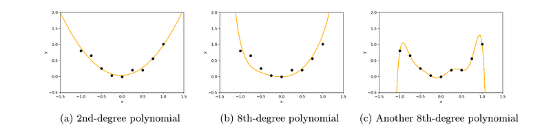
Here we have a 2nd-degree polynomial fit and two different 8th-degree polynomials, given by the following equations:
这里有一个二阶多项式拟合和两个不同的八阶多项式,其方程如下:
Figure a:
y
^
=
0.04
+
0.04
x
+
0.9
x
2
\hat {y} = 0.04 + 0.04x + 0.9x^2
y^=0.04+0.04x+0.9x2
Figure b:
y
^
=
−
0.01
+
0.01
x
+
0.8
x
2
+
0.5
x
3
−
0.1
x
4
−
0.1
x
5
+
0.3
x
6
−
0.3
x
7
+
0.2
x
8
\hat {y} = -0.01 + 0.01x + 0.8x^2 + 0.5x^3 - 0.1x^4 - 0.1x^5 + 0.3x^6 - 0.3x^7 + 0.2x^8
y^=−0.01+0.01x+0.8x2+0.5x3−0.1x4−0.1x5+0.3x6−0.3x7+0.2x8
Figure c:
y
^
=
−
0.01
+
0.57
x
+
2.67
x
2
−
4.08
x
3
−
12.25
x
4
+
7.41
x
5
+
24.87
x
6
−
3.79
x
7
−
14.38
x
8
\hat {y} = -0.01 + 0.57x + 2.67x^2 - 4.08x^3 - 12.25x^4 + 7.41x^5 + 24.87x^6 - 3.79x^7 - 14.38x^8
y^=−0.01+0.57x+2.67x2−4.08x3−12.25x4+7.41x5+24.87x6−3.79x7−14.38x8
The first two (which are “simpler” functions) will most likely generalize better to new data, while the third one (a more complex function) is clearly overfitting the training data. How is this complexity reflected in the norm?
前两个(更简单的函数)更有可能在新数据上表现良好,而第三个(更复杂的函数)显然过拟合了训练数据。这种复杂性是如何在范数中体现的呢?
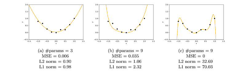
As we can see, line [c] has a mean squared error of 0, but its norms are quite high. Lines [a] and [b], instead, have a slightly higher MSE but their norms are much lower:
我们可以看到,线 [c] 的均方误差为 0,但其范数相当高。相反,线 [a] 和 [b] 的均方误差略高,但其范数要低得多:
- Line [a] has lower norms because it has significantly fewer parameters compared to [c]
线 [a] 的范数较低,因为它比 [c] 的参数少得多 - Line [b] has lower norms because despite having the same number of parameters, they are all much smaller than [c]
线 [b] 的范数较低,尽管它与 [c] 的参数数量相同,但其参数值要小得多
From this we can conclude that by adding the L1 or L2 norm to our minimization objective, we can encourage simpler functions with lower weights, which will have a regularization effect and help our model to better generalize on new data.
从这一点我们可以得出结论,通过将 L1 或 L2 范数添加到我们的最小化目标中,我们可以鼓励使用更小权重的更简单函数,这将产生正则化效果,并帮助我们的模型在新数据上表现更好。
What’s the difference between the L1 norm and the L2 norm?
L1 范数和 L2 范数区别
We’ve already seen that to reduce the complexity of a function we can either drop some weights entirely (setting them to zero), or make all weights as small as possible, which brings us to the difference between L1 and L2.
我们已经看到,为了减少函数的复杂性,我们可以完全去掉一些权重(将它们设置为零),或者使所有权重尽可能小,这让我们来到了 L1 和 L2 的区别。
To understand how they operate differently, let’s have a look at how they change depending on the value of the weights.
为了理解它们如何不同地运作,让我们看看它们如何随着权重值的变化而变化。
On the left we have a plot of the L1 and L2 norm for a given weight
w
w
w. On the right, we have the corresponding graph for the slope of the norms. As we can see, both L1 and L2 increase for increasing absolute values of
w
w
w. However, while the L1 norm increases at a constant rate, the L2 norm increases exponentially.
在左边,我们有一个给定权重
w
w
w 的 L1 和 L2 范数的图。在右边,我们有范数斜率的相应图。我们可以看到,随着
w
w
w 的绝对值增加,L1 和 L2 范数都会增加。然而,尽管 L1 范数以恒定速率增加,但 L2 范数呈指数增长。
This is important because, as we know, when doing gradient descent we’ll update our weights based on the derivative of the loss function. So if we’ve included a norm in our loss function, thederivative of the norm will determine how the weights get updated.
这很重要,因为正如我们所知,在进行梯度下降时,我们会根据损失函数的导数来更新权重。因此,如果我们已经在损失函数中包含了范数,那么范数的导数将决定权重如何更新。
We can see that with theL2 normas
w
w
w gets smaller so does the slope of the norm, meaning that the updates will also become smaller and smaller. When the weights are close to 0 the updates will have become so small as to be almost negligible, so it’s unlikely that the weights will ever become 0.
我们可以看到,随着
w
w
w 变小,L2 范数的斜率也会变小,这意味着更新也会变得越来越小。当权重接近 0 时,更新将变得如此之小,几乎可以忽略不计,因此权重几乎不可能变为 0。
On the other hand, with theL1 normthe slope is constant. This means that as
w
w
w gets smaller the updates don’t change, so we keep getting the same “reward” for making the weights smaller. Therefore, the L1 norm is much more likely to reduce some weights to 0.
另一方面,L1 范数的斜率是恒定的。这意味着随着
w
w
w 变小,更新不会改变,因此我们继续获得使权重变小的相同 “奖励”。因此,L1 范数更有可能将一些权重减少到 0。
To recap:
总结:
- TheL1 norm will drive some weights to 0, inducing sparsity in the weights. This can be beneficial formemory efficiencyor whenfeature selectionis needed (i.e., we want to select only certain weights).
L1 范数会将一些权重驱动至 0,从而在权重中引入稀疏性。这在需要内存效率或进行特征选择时是有益的(即,我们只想选择某些权重)。 - TheL2 norminstead willreduce all weights but not all the way to 0. This is less memory efficient but can be useful if we want/need to retain all parameters.
相比之下,L2 范数会减小所有权重,但不会完全减至 0。这在内存效率方面稍差,但如果我们希望 / 需要保留所有参数时,它可能是有用的。
Vector Norms: A Quick Guide
向量范数:快速指南
Written by Parul Pandey
Updated By Brennan Whitfield | Apr 28, 2025
A vector norm is a function that measures the size or magnitude of a vector by quantifying its length from the origin. Vector norms are an important concept to machine learning. This guide breaks down the idea behind the
L
1
L^1
L1,
L
2
L^2
L2,
L
∞
L^\infty
L∞ and
L
p
L^p
Lp norms.
向量范数是一种函数,通过量化向量从原点出发的长度,来衡量向量的大小或幅值。向量范数是机器学习中的重要概念。本指南将详细解析
L
1
L^1
L1、
L
2
L^2
L2、
L
∞
L^\infty
L∞ 和
L
p
L^p
Lp 范数的基本原理。
Summary: A vector norm is a type of function that measures the size or magnitude of a vector. It helps quantify a vector’s length and plays a key role in machine learning for tasks like loss functions, regularization and calculating distances between data points.
摘要:向量范数是一类用于衡量向量大小或幅值的函数。它有助于量化向量的长度,在机器学习中发挥关键作用,适用于损失函数定义、正则化以及数据点间距离计算等任务。
Many applications like information retrieval, personalization, document categorization, image processing, and so on, rely on the computation of similarity or dissimilarity between items. Two items are considered similar if the distance between them is small, and vice versa.
许多应用场景(如信息检索、个性化推荐、文档分类、图像处理等)都依赖于物品间相似度或相异度的计算。若两个物品间的距离较小,则认为它们相似,反之则不相似。
So, how do we calculate this distance? Well, each data object (item) can be thought of as an
n
n
n-dimensional vector where the dimensions are the attributes (features) in the data. The vector representations thereby make it possible to compute the distance between pairs using the standard vector-based similarity measures like the Manhattan distance or Euclidean distance, to name two. During such calculations, norms come up. Vector norms occupy an important space in the context of machine learning, so in this article, we’ll first work to understand the basics of a norm and its properties and then go over some of the most common vector norms.
那么,我们如何计算这种距离呢?每个数据对象(物品)都可以被视为一个
n
n
n 维向量,其中维度对应数据中的属性(特征)。通过向量表示,我们可以使用标准的基于向量的相似度度量方法(例如曼哈顿距离或欧几里得距离,仅举两例)来计算成对物品间的距离。在这些计算过程中,范数会被频繁用到。向量范数在机器学习领域占据重要地位,因此本文将首先帮助读者理解范数的基础概念及其性质,然后详细介绍几种最常用的向量范数。
Common Vector Norms in Machine Learning
机器学习中常见的向量范数
-
L
1
L^1
L1 / Manhattan Norm
L 1 L^1 L1 范数 / 曼哈顿范数 -
L
2
L^2
L2 / Euclidean Norm
L 2 L^2 L2 范数 / 欧几里得范数 -
L
∞
L^\infty
L∞ Norm
L ∞ L^\infty L∞ 范数 -
L
p
L^p
Lp Norm
L p L^p Lp 范数
What Is a Norm?
什么是范数?
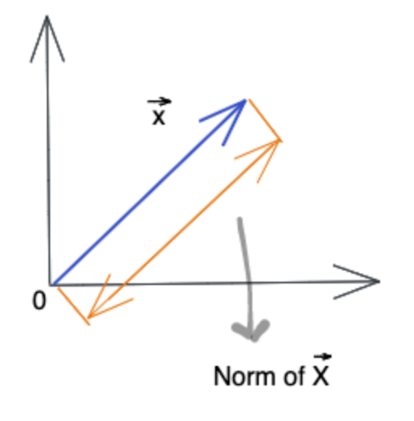
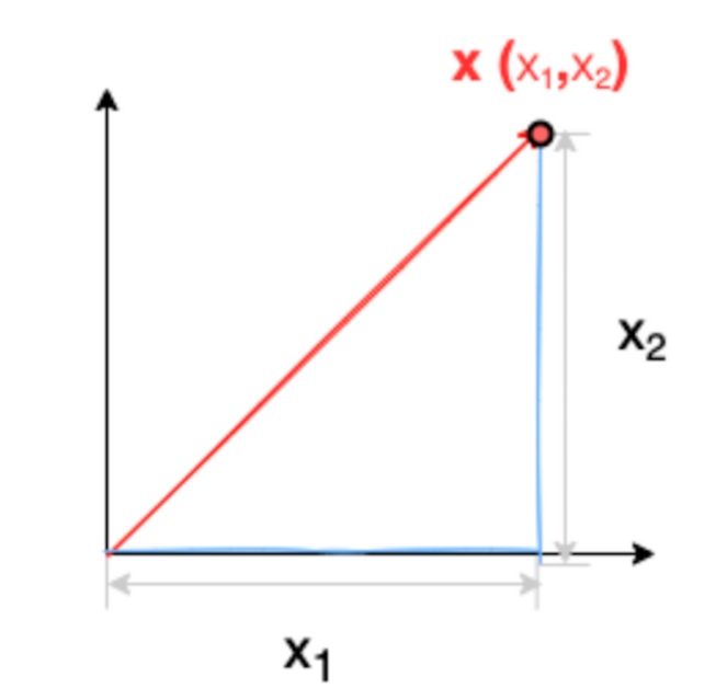
A norm is a way to measure the size of a vector, a matrix, or a tensor. In other words, norms are a class of functions that enable us to quantify the magnitude of a vector. For instance, the norm of a vector
X
X
X drawn below is a measure of its length from origin.
范数是一种衡量向量、矩阵或张量大小的方法。换句话说,范数是一类函数,能够让我们量化向量的幅值。例如,下图中向量
X
X
X 的范数,就是其从原点出发的长度度量。
The subject of norms comes up on many occasions in the context of machine learning:
范数相关内容在机器学习中会在多种场景下出现:
- When defining loss functions, i.e., the distance between the actual and predicted values
定义损失函数时,即衡量真实值与预测值之间的距离 - As a regularization method in machine learning, e.g., ridge and lasso regularization methods.
作为机器学习中的正则化方法,例如岭回归和套索回归正则化方法 - Even algorithms like support vector machine (SVM) use the concept of the norm to calculate the distance between the discriminant and each support-vector.
甚至支持向量机(SVM)等算法也会利用范数概念,计算判别面与每个支持向量之间的距离
How Do We Represent Norms?
范数表示
The norm of any vector
X
X
X is denoted by a double bar around it and is written as follows:
任意向量
X
X
X 的范数用双竖线包裹表示,格式如下:
norm of vector
x
x
x:
∥
x
∥
\|x\|
∥x∥
向量
x
x
x 的范数:
∥
x
∥
\|x\|
∥x∥
What Are the Properties of a Norm?
范数的性质
Consider two vectors
X
X
X and
Y
Y
Y, having the same size and scalar. A function is considered a norm only if it satisfies the following properties:
假设有两个同维度向量
X
X
X 和
Y
Y
Y,以及一个标量。一个函数要被称为范数,必须满足以下性质:
- Non-negativity: It should always be non-negative.
非负性:范数值始终非负。 - Definiteness: It is zero if and only if the vector is zero, i.e., zero vector.
确定性:当且仅当向量为零向量时,范数值为零。 - Triangle inequality: The norm of a sum of two vectors is no more than the sum of their norms (
∥
X
+
Y
∥
≤
∥
x
∥
+
∥
Y
∥
\|X+Y\| \leq \|x\| + \|Y\|
∥X+Y∥≤∥x∥+∥Y∥).
三角不等式:两个向量和的范数不大于它们各自范数的和( ∥ X + Y ∥ ≤ ∥ x ∥ + ∥ Y ∥ \|X+Y\| \leq \|x\| + \|Y\| ∥X+Y∥≤∥x∥+∥Y∥)。 - Homogeneity: Multiplying a vector by a real scalar multiplies the norm of the vector by the absolute value of the scalar (for any real scalar
λ
\lambda
λ,
∥
λ
X
∥
=
∣
λ
∣
∥
x
∥
\|\lambda X\| = |\lambda| \|x\|
∥λX∥=∣λ∣∥x∥).
齐次性:将向量乘以一个实标量,向量的范数会乘以该标量的绝对值(对于任意实标量 λ \lambda λ, ∥ λ X ∥ = ∣ λ ∣ ∥ x ∥ \|\lambda X\| = |\lambda| \|x\| ∥λX∥=∣λ∣∥x∥)。
Let’s see these qualities represented mathematically.
下面我们用数学形式展示这些性质。
Non-Negativity
非负性
∥ x ∥ ≥ 0 \|x\| \geq 0 ∥x∥≥0
Definiteness
确定性
∥ x ∥ = 0 if and only if x = 0 \|x\| = 0 \quad \text {if and only if} \quad x = 0 ∥x∥=0if and only ifx=0
Triangle Inequality
三角不等式
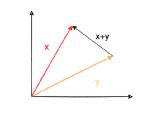
∥ x + y ∥ ≤ ∥ x ∥ + ∥ y ∥ \|x+y\| \leq \|x\| + \|y\| ∥x+y∥≤∥x∥+∥y∥
Homogeneity
齐次性
∥ λ x ∥ = ∣ λ ∣ ∥ x ∥ , where λ ∈ R \|\lambda x\| = |\lambda| \|x\|, \quad \text {where } \lambda \in \mathbb {R} ∥λx∥=∣λ∣∥x∥,where λ∈R
Any real value function of a vector that satisfies the above four properties is called a norm.
任何满足上述四个性质的向量实值函数,都可称为范数。
What Are Some Standard Norms?
常见的标准范数
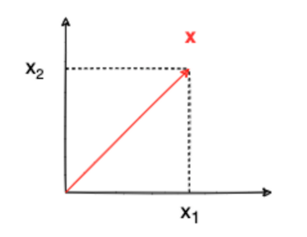
A lot of functions can be defined that satisfy the properties above. Consider a two-dimensional column vector
X
X
X as follows:
我们可以定义许多满足上述性质的函数。假设存在一个二维列向量
X
X
X 如下:
x = [ x 1 x 2 ] x = \begin {bmatrix} x_1 \\ x_2 \end {bmatrix} x=[x1x2]
We can now calculate some standard norms for
X
X
X, starting with the
L
1
L^1
L1 norm.
下面我们从
L
1
L^1
L1 范数开始,计算向量
X
X
X 的几种标准范数。
What Is the L 1 L^1 L1 Norm / Manhattan Norm?
L 1 L^1 L1 范数 / 曼哈顿范数
The
L
1
L^1
L1 norm is defined as the sum of the absolute values of the components of a given vector. Since we have a vector
X
X
X with only two components, the
L
1
L^1
L1 norm of
X
X
X can be written as:
L
1
L^1
L1 范数定义为给定向量各分量绝对值的和。由于我们的向量
X
X
X 仅有两个分量,其
L
1
L^1
L1 范数可表示为:
∥ x ∥ 1 = ∣ x 1 ∣ + ∣ x 2 ∣ \|x\|_1 = |x_1| + |x_2| ∥x∥1=∣x1∣+∣x2∣
Notice the representation with one written as a subscript. This norm is also called the Manhattan or the taxicab norm, inspired by the borough of Manhattan in New York. The
L
1
L^1
L1 norm is typically the distance a taxi will have to drive from the origin to point
X
X
X.
注意下标为 1 的表示方式。该范数也被称为曼哈顿范数或出租车范数,其命名灵感来自美国纽约的曼哈顿区。
L
1
L^1
L1 范数通常对应出租车从原点行驶到点
X
X
X 所需的距离。
Mathematical Notation
数学表示
The
L
1
L^1
L1 norm can be mathematically written as:
L
1
L^1
L1 范数的数学表达式为:
∥
x
∥
1
=
∑
i
=
1
n
∣
x
i
∣
\|x\|_1 = \sum_{i=1}^{n} |x_i|
∥x∥1=i=1∑n∣xi∣
where
X
∈
R
n
X \in \mathbb {R}^n
X∈Rn is a vector of dimension
n
n
n with coordinates
x
i
x_i
xi.
其中
X
∈
R
n
X \in \mathbb {R}^n
X∈Rn 是一个
n
n
n 维向量,
x
i
x_i
xi 是其各分量坐标。
What Are the Properties of the L 1 L^1 L1 / Manhattan Norm?
L 1 L^1 L1 范数 / 曼哈顿范数的性质
- The
L
1
L^1
L1 norm is used in situations when it is helpful to distinguish between zero and non-zero values.
当需要区分零值和非零值时,可使用 L 1 L^1 L1 范数。 - The
L
1
L^1
L1 norm increases proportionally with the components of the vector.
L 1 L^1 L1 范数随向量分量的增大而成比例增长。 - It is used in Lasso (Least Absolute Shrinkage and Selection Operator) regression, which involves adding the
L
1
L^1
L1 norm of the coefficient as a penalty term to the loss function.
它被应用于套索回归(Lasso,最小绝对收缩与选择算子)中,即将系数的 L 1 L^1 L1 范数作为惩罚项加入损失函数。
What Is the L 2 L^2 L2 Norm / Euclidean Norm?
L 2 L^2 L2 范数 / 欧几里得范数
L
2
L^2
L2 is the most commonly used norm and the one most encountered in real life. The
L
2
L^2
L2 norm measures the shortest distance from the origin. It is defined as the root of the sum of the squares of the components of the vector. So, for our given vector
X
X
X, the
L
2
L^2
L2 norm would be:
L
2
L^2
L2 范数是最常用的范数,也是现实生活中最易遇到的范数。它衡量的是从原点到向量点的最短距离,定义为向量各分量平方和的平方根。因此,对于给定向量
X
X
X,其
L
2
L^2
L2 范数为:
∥ x ∥ 2 = x 1 2 + x 2 2 \|x\|_2 = \sqrt {x_1^2 + x_2^2} ∥x∥2=x12+x22
The
L
2
L^2
L2 norm is so common that it is sometimes also denoted without any subscript:
L
2
L^2
L2 范数的使用频率极高,因此有时也会省略下标表示:
∥ x ∥ = x 1 2 + x 2 2 \|x\| = \sqrt {x_1^2 + x_2^2} ∥x∥=x12+x22
The
L
2
L^2
L2 norm is also known as the Euclidean norm after the famous Greek mathematician, often referred to as the founder of geometry. The Euclidean norm essentially means we are referring to the Euclidean distance.
L
2
L^2
L2 范数也被称为欧几里得范数,以著名的希腊数学家(通常被认为是几何学创始人)欧几里得命名。欧几里得范数本质上就是指欧几里得距离。
Mathematical Notation
数学表示
The
L
2
L^2
L2 norm can be mathematically written as:
L
2
L^2
L2 范数的数学表达式为:
∥
x
∥
2
=
∑
i
=
1
n
∣
x
i
∣
2
\|x\|_2 = \sqrt {\sum_{i=1}^{n} |x_i|^2}
∥x∥2=i=1∑n∣xi∣2
where
X
∈
R
n
X \in \mathbb {R}^n
X∈Rn is a vector of dimension
n
n
n with coordinates
x
i
x_i
xi.
其中
X
∈
R
n
X \in \mathbb {R}^n
X∈Rn 是一个
n
n
n 维向量,
x
i
x_i
xi 是其各分量坐标。
What Are the Properties of the L 2 L^2 L2 Norm?
L 2 L^2 L2 范数的性质
- The
L
2
L^2
L2 norm is the most commonly used one in machine learning.
L 2 L^2 L2 范数是机器学习中最常用的范数。 - Since it entails squaring of each component of the vector, it is not robust to outliers.
由于它需要对向量的每个分量进行平方运算,因此对异常值不稳健。 - Since the
L
2
L^2
L2 norm squares each component, very small components become even smaller. For example,
(
0.1
)
2
=
0.01
(0.1)^2 = 0.01
(0.1)2=0.01.
由于 L 2 L^2 L2 范数会对各分量进行平方,极小的分量会变得更小。例如, ( 0.1 ) 2 = 0.01 (0.1)^2 = 0.01 (0.1)2=0.01。 - It is used in ridge regression, which involves adding the
L
2
L^2
L2 norm of the coefficient as a penalty term to the loss function.
它被应用于岭回归中,即将系数的 L 2 L^2 L2 范数作为惩罚项加入损失函数。
What Is the L ∞ L^\infty L∞ / Max Norm?
L ∞ L^\infty L∞ 范数 / 最大范数
The
L
∞
L^\infty
L∞ norm is defined as the absolute value of the largest component of the vector, or the maximum absolute value among the vector’s components. Therefore, it is also called the max norm. So, continuing with our example of a 2D vector
X
X
X having two components (i.e.,
x
1
x_1
x1 and
x
2
x_2
x2, where
x
2
>
x
1
x_2 > x_1
x2>x1), the
L
∞
L^\infty
L∞ norm would simply be the absolute value of
x
2
x_2
x2:
∥
x
∥
∞
=
∣
x
2
∣
\|x\|_\infty = |x_2|
∥x∥∞=∣x2∣.
L
∞
L^\infty
L∞ 范数定义为向量中最大分量的绝对值,或向量各分量绝对值中的最大值。因此,它也被称为最大范数。沿用之前的二维向量
X
X
X 示例(含两个分量
x
1
x_1
x1 和
x
2
x_2
x2,且
x
2
>
x
1
x_2 > x_1
x2>x1),其
L
∞
L^\infty
L∞ 范数即为
x
2
x_2
x2 的绝对值:
∥ x ∥ ∞ = ∣ x 2 ∣ \|x\|_\infty = |x_2| ∥x∥∞=∣x2∣
Mathematical Notation
数学表示
The
L
∞
L^\infty
L∞ norm can be mathematically written as:
L
∞
L^\infty
L∞ 范数的数学表达式为:
∥
x
∥
∞
=
max
i
(
∣
x
i
∣
)
\|x\|_\infty = \max_{i} (|x_i|)
∥x∥∞=imax(∣xi∣)
What Are the Properties of the Max Norm?
最大范数的性质
- The
L
∞
L^\infty
L∞ norm simplifies to the absolute value of the largest element in the vector.
L ∞ L^\infty L∞ 范数可简化为向量中最大元素的绝对值。
What Is the L p L^p Lp Norm?
L p L^p Lp 范数
We can now generalize to the idea of what is known as the
p
p
p-norm. In a way, we can derive all other norms from the
p
p
p-norm by varying the values of
p
p
p. That is to say, if you substitute the value of
p
p
p with one, two, and
∞
\infty
∞ respectively in the formula below, you’ll obtain
L
1
L^1
L1,
L
2
L^2
L2, and
L
∞
L^\infty
L∞ norms.
我们可以将范数概念推广到
p
p
p- 范数(即
L
p
L^p
Lp 范数)。在某种程度上,通过改变
p
p
p 的取值,我们可以从
p
p
p- 范数推导出其他所有范数。也就是说,在下面的公式中,分别将
p
p
p 取值为 1、2 和
∞
\infty
∞,即可得到
L
1
L^1
L1、
L
2
L^2
L2 和
L
∞
L^\infty
L∞ 范数。
Mathematical Notation
数学表示
The
L
p
L^p
Lp norm can be mathematically written as:
L
p
L^p
Lp 范数的数学表达式为:
∥
x
∥
p
=
(
∑
i
=
1
n
∣
x
i
∣
p
)
1
/
p
,
where
p
>
0
\|x\|_p = \left ( \sum_{i=1}^{n} |x_i|^p \right)^{1/p}, \quad \text {where } p > 0
∥x∥p=(i=1∑n∣xi∣p)1/p,where p>0
An important point to remember here is that each of the norms above fulfills the properties of the norms mentioned in the beginning.
需要注意的是,上述每种范数都满足前文提到的范数基本性质。
What happens when p p p equals zero?
当 p = 0 p = 0 p=0 时会发生什么?
When this happens, we might want to call the value
L
0
L^0
L0 “norm” (however, it’s not technically a norm because it doesn’t satisfy the homogeneity property). The so-called “
L
0
L^0
L0 norm” is useful when we want to know the number of non-zero components in a vector. This means sparsity can be modeled via the
L
0
L^0
L0 “norm.”
此时,我们可能会将其称为
L
0
L^0
L0“范数”(但严格来说,它并不是真正的范数,因为它不满足齐次性)。所谓的 “
L
0
L^0
L0 范数” 在我们需要知道向量中非零分量的数量时非常有用,这意味着可以通过
L
0
L^0
L0“范数” 来建模稀疏性。
∥ x ∥ 0 = number of non-zero entries in X \|x\|_0 = \text {number of non-zero entries in } X ∥x∥0=number of non-zero entries in X
So for instance if we have a vector
x
=
[
2
4
0
]
\mathbf {x} = \begin {bmatrix} 2 \\ 4 \\ 0 \end {bmatrix}
x=
240
,
∥
x
∥
0
=
2
\|\mathbf {x}\|_0 = 2
∥x∥0=2 (no of non zero elements)
举个例子,若我们有一个向量
x
=
[
2
4
0
]
\mathbf {x} = \begin {bmatrix} 2 \\ 4 \\ 0 \end {bmatrix}
x=
240
,则其
L
0
L^0
L0 范数
∥
x
∥
0
=
2
\|\mathbf {x}\|_0 = 2
∥x∥0=2(即非零元素的数量)
L 0 L^0 L0 范数只统计非零元素的数量,与向量是行形式还是列形式无关。
Example: X = [ 2 4 0 ] X = \begin {bmatrix} 2 & 4 & 0 \end {bmatrix} X=[240], ∥ x ∥ 0 = 2 \|x\|_0 = 2 ∥x∥0=2
示例: X = [ 2 4 0 ] X = \begin {bmatrix} 2 & 4 & 0 \end {bmatrix} X=[240],则 ∥ x ∥ 0 = 2 \|x\|_0 = 2 ∥x∥0=2
Sparsity is an important concept in machine learning, as it helps to improve robustness and prevent overfitting.
稀疏性是机器学习中的重要概念,有助于提升模型的稳健性并防止过拟合。
Vector Norms Summed Up
向量范数总结
This article looked at the concept of a vector norm, its properties, and some commonly used norms that we encounter in machine learning.
本文介绍了向量范数的概念、性质,以及机器学习中常见的几种向量范数。
You may also find these resources on linear algebra useful for understanding vector norms further.
你还可以参考以下线性代数相关资源,以进一步理解向量范数。
- Introduction to Linear Algebra (Gilbert Strang, 2): Strang, Gilbert: 9780980232776: Amazon.com: Books
https://www.amazon.com/Introduction-Linear-Algebra-Gilbert-Strang/dp/0980232775/ - https://wwwyoutube.com/playlist?list=PLUl4u3cNGP63oMNUHXqIUcrkS2PivhN3k
Frequently Asked Questions
常见问题
What is a vector norm?
向量范数
A vector norm is a function that measures the size or magnitude of a vector by quantifying its length from the origin. To be a vector norm, a function must satisfy the following properties: non-negativity, definiteness, triangle inequality and homogeneity.
向量范数是一种通过量化向量从原点出发的长度,来衡量向量大小或幅值的函数。一个函数要成为向量范数,必须满足以下性质:非负性、确定性、三角不等式和齐次性。
Why are vector norms important in machine learning?
机器学习中的向量范数
Vector norms are important in machine learning because they are used to calculate distances between data points, define loss functions, apply regularization techniques and are involved in algorithms like support vector machine (SVM).
向量范数在机器学习中至关重要,因为它们可用于计算数据点间的距离、定义损失函数、应用正则化技术,并且在支持向量机(SVM)等算法中也有应用。
范数(Norm)理论与应用
范数定义与性质
范数是数学中用于度量向量或矩阵 “大小” 的函数,其概念源于几何距离,且拓展了数乘运算的适配性。在严格数学定义中,向量范数需满足以下三条基本性质:
1.非负性:对任意向量
x
x
x,有
∥
x
∥
≥
0
\|x\| \geq 0
∥x∥≥0;且当且仅当
x
x
x 为零向量(
x
=
0
x = 0
x=0)时,
∥
x
∥
=
0
\|x\| = 0
∥x∥=0;
2.齐次性:对任意标量
a
a
a 和任意向量
x
x
x,有
∥
a
x
∥
=
∣
a
∣
⋅
∥
x
∥
\|ax\| = |a| \cdot \|x\|
∥ax∥=∣a∣⋅∥x∥(标量的绝对值与向量范数成正比);
3.三角不等式:对任意向量
x
x
x 和
y
y
y,有
∥
x
+
y
∥
≤
∥
x
∥
+
∥
y
∥
\|x + y\| \leq \|x\| + \|y\|
∥x+y∥≤∥x∥+∥y∥(两向量和的范数不超过各自范数之和)。
矩阵范数是向量范数的延伸,除满足上述三条性质外,还需额外满足相容性:对任意两个可乘矩阵(即 A A A 的列数等于 B B B 的行数) A A A 和 B B B,有 ∥ A B ∥ ≤ ∥ A ∥ ⋅ ∥ B ∥ \|AB\| \leq \|A\| \cdot \|B\| ∥AB∥≤∥A∥⋅∥B∥。范数的关键价值在于:将高维空间中无法直接感知的向量 / 矩阵,映射为可量化的实数,为距离度量、收敛性判断、极限求解等后续操作提供数学基础。
引入范数的意义
在三维及以下空间中,几何图形可通过直观感知分析,但高维空间(如机器学习中的特征空间)缺乏具象化工具,范数通过统一映射规则填补了这一空白,具体意义体现在两方面:
1.解决 “大小比较” 问题:一维实数可通过数值直接比较大小,但二维及以上空间的向量无天然评判标准(如向量
(
1
,
3
)
(1,3)
(1,3) 与
(
2
,
2
)
(2,2)
(2,2) 无法直接判断 “更大”),范数通过数学规则将向量 / 矩阵转化为单值,实现 “大小” 量化;
2.支撑关键数学操作:借助范数可定义向量间的距离(如两向量
x
,
y
x,y
x,y 的距离可表示为
∥
x
−
y
∥
\|x - y\|
∥x−y∥),进而支撑逼近程度分析、迭代算法收敛性判断(如数值分析中,通过范数度量迭代前后结果的差值,当差值小于阈值时判定收敛)。
向量范数的类型与特性
L p L^p Lp 范数
L
p
L^p
Lp 范数是一组具有通用性的向量范数,其数学表达式为:
∥
x
∥
p
=
(
∑
i
=
1
n
∣
x
i
∣
p
)
1
p
(
p
≥
1
)
\|x\|_p = \left ( \sum_{i=1}^{n} |x_i|^p \right)^{\frac {1}{p}} \quad (p \geq 1)
∥x∥p=(i=1∑n∣xi∣p)p1(p≥1)
其中
x
=
(
x
1
,
x
2
,
…
,
x
n
)
x = (x_1, x_2, \dots, x_n)
x=(x1,x2,…,xn) 为
n
n
n 维向量,
p
p
p 的取值直接决定范数的度量逻辑,主要特性可通过三维空间直观体现:当
∥
x
∥
p
=
1
\|x\|_p = 1
∥x∥p=1 时,
p
=
2
p = 2
p=2 对应球面、
p
→
∞
p \to \infty
p→∞ 对应立方体、
p
=
1
p = 1
p=1 对应正八面体。
需注意:当
p
<
1
p < 1
p<1 时,上述表达式不满足三角不等式,不属于严格意义上的范数。例如
p
=
0.5
p = 0.5
p=0.5 时,二维向量
(
1
,
4
)
(1,4)
(1,4)、
(
4
,
1
)
(4,1)
(4,1)、
(
1
,
9
)
(1,9)
(1,9) 满足:
∥
(
1
,
4
)
−
(
4
,
1
)
∥
0.5
+
∥
(
4
,
1
)
−
(
1
,
9
)
∥
0.5
<
∥
(
1
,
4
)
−
(
1
,
9
)
∥
0.5
\|(1,4) - (4,1)\|_{0.5} + \|(4,1) - (1,9)\|_{0.5} < \|(1,4) - (1,9)\|_{0.5}
∥(1,4)−(4,1)∥0.5+∥(4,1)−(1,9)∥0.5<∥(1,4)−(1,9)∥0.5
L0 范数
当
p
=
0
p = 0
p=0 时,
L
p
L^p
Lp 范数无法直接套用(数学中
0
0
0^0
00 无意义),因此 L0 范数的严格定义为向量中非零元素的个数,而非原始表达式的延伸:
∥
x
∥
0
=
向量
x
中非零元素的数量
\|x\|_0 = \text {向量} x \text {中非零元素的数量}
∥x∥0=向量x中非零元素的数量
L0 范数的主要应用是稀疏编码与特征选择,对应的优化问题为
min
∥
x
∥
0
s.t.
A
x
=
b
\min \|x\|_0 \quad \text {s.t.} \quad Ax = b
min∥x∥0s.t.Ax=b(在约束
A
x
=
b
Ax = b
Ax=b 下最小化非零元素个数)。但该问题属于NP 难问题(求解复杂度极高),实际应用中常将其放宽为 L1 范数或 L2 范数优化,以降低求解难度。
L1 范数
L1 范数是
p
=
1
p = 1
p=1 时的
L
p
L^p
Lp 范数,数学表达式为:
∥
x
∥
1
=
∑
i
=
1
n
∣
x
i
∣
\|x\|_1 = \sum_{i=1}^{n} |x_i|
∥x∥1=i=1∑n∣xi∣
其物理意义是向量所有元素的绝对值之和,也被称为 “曼哈顿距离” 或 “最小绝对误差”。基于 L1 范数可定义两向量的差异度量 ——绝对误差和(Sum of Absolute Difference, SAD):
SAD
(
x
,
y
)
=
∑
i
=
1
n
∣
x
i
−
y
i
∣
\text {SAD}(x,y) = \sum_{i=1}^{n} |x_i - y_i|
SAD(x,y)=i=1∑n∣xi−yi∣
L1 范数的关键特性是能产生稀疏解:其优化问题
min
∥
x
∥
1
s.t.
A
x
=
b
\min \|x\|_1 \quad \text {s.t.} \quad Ax = b
min∥x∥1s.t.Ax=b 的解中,大量元素会趋近于零。这一特性使其成为特征选择的重要工具,例如在用户行为分类任务中,可过滤身高、体重等与分类无关的特征,仅保留关键维度。
L2 范数
L2 范数是应用最广泛的向量范数,对应
p
=
2
p = 2
p=2 时的
L
p
L^p
Lp 范数,数学表达式为:
∥
x
∥
2
=
(
∑
i
=
1
n
x
i
2
)
1
2
\|x\|_2 = \left ( \sum_{i=1}^{n} x_i^2 \right)^{\frac {1}{2}}
∥x∥2=(i=1∑nxi2)21
其物理意义等价于 “欧氏距离”(即向量元素平方和的平方根),可定义两向量的平方差和(Sum of Squared Difference, SSD):
SSD
(
x
,
y
)
=
∑
i
=
1
n
(
x
i
−
y
i
)
2
\text {SSD}(x,y) = \sum_{i=1}^{n} (x_i - y_i)^2
SSD(x,y)=i=1∑n(xi−yi)2
L2 范数的主要应用是模型正则化:将其作为正则化项加入目标函数,可限制模型参数的绝对值大小,避免参数过大导致的模型复杂度过高,从而抑制过拟合、提升泛化能力。这种结合 L2 范数的回归方法被称为 “岭回归(Ridge Regression)” 或 “权重衰减(Weight Decay)”,原理是通过缩小参数取值,降低模型对训练数据噪声的敏感性,使其更倾向于学习数据的通用规律。
注:“s.t.” 是 “subject to” 的缩写,意为 “受限于…”,常用于优化问题的约束条件表述。
无穷范数
当
p
→
∞
p \to \infty
p→∞ 时,
L
p
L^p
Lp 范数收敛为无穷范数,数学表达式为:
∥
x
∥
∞
=
max
1
≤
i
≤
n
∣
x
i
∣
\|x\|_\infty = \max_{1 \leq i \leq n} |x_i|
∥x∥∞=1≤i≤nmax∣xi∣
其物理意义是向量所有元素绝对值中的最大值,主要应用场景是需关注向量 “极端值” 的场景,例如误差分析中对 “最大偏差” 的度量(如控制系统中,需确保某一维度的误差不超过阈值)。
矩阵范数的类型与计算
设 A A A 为 m × n m \times n m×n 矩阵(行维度 m m m,列维度 n n n),元素记为 a i , j a_{i,j} ai,j(第 i i i 行第 j j j 列),常见矩阵范数的定义与计算规则如下:
矩阵 1 - 范数(列模)
矩阵 1 - 范数的数学表达式为:
∥
A
∥
1
=
max
j
∑
i
=
1
m
∣
a
i
,
j
∣
\|A\|_1 = \max_{j} \sum_{i=1}^{m} |a_{i,j}|
∥A∥1=jmaxi=1∑m∣ai,j∣
计算逻辑:对矩阵的每一列,先求该列所有元素绝对值的和(即列向量的 L1 范数),再取所有列和中的最大值。其物理意义反映矩阵列向量的 “累积强度”,例如在信号传输中,可用于度量某一列信号的最大 “总振幅”。
矩阵 2 - 范数(谱模)
矩阵 2 - 范数的数学表达式为:
∥
A
∥
2
=
λ
max
(
A
T
A
)
\|A\|_2 = \sqrt {\lambda_{\max}(A^T A)}
∥A∥2=λmax(ATA)
其中
A
T
A^T
AT 为
A
A
A 的转置矩阵,
λ
max
(
A
T
A
)
\lambda_{\max}(A^T A)
λmax(ATA) 表示矩阵
A
T
A
A^T A
ATA 的最大特征值。该范数也被称为 “谱模”,其值与矩阵的谱特性(特征值分布)直接相关,主要应用是度量线性变换的 “最大拉伸强度”(如信号处理中,可表示矩阵对输入信号的最大放大倍数),在图像处理、控制系统等领域应用广泛。
矩阵∞- 范数(行模)
矩阵∞- 范数的数学表达式为:
∥
A
∥
∞
=
max
i
∑
j
=
1
n
∣
a
i
,
j
∣
\|A\|_\infty = \max_{i} \sum_{j=1}^{n} |a_{i,j}|
∥A∥∞=imaxj=1∑n∣ai,j∣
计算逻辑:对矩阵的每一行,先求该行所有元素绝对值的和(即行向量的 L1 范数),再取所有行和中的最大值。其物理意义反映矩阵行向量的 “累积强度”,例如在数据分类中,可用于度量某一行特征的最大 “总贡献度”。
矩阵 F - 范数(Frobenius 范数)
矩阵 F - 范数的数学表达式为:
∥
A
∥
F
=
(
∑
i
=
1
m
∑
j
=
1
n
∣
a
i
,
j
∣
2
)
1
2
=
Tr
(
A
A
T
)
\|A\|_F = \left ( \sum_{i=1}^{m} \sum_{j=1}^{n} |a_{i,j}|^2 \right)^{\frac {1}{2}} = \sqrt {\text {Tr}(A A^T)}
∥A∥F=(i=1∑mj=1∑n∣ai,j∣2)21=Tr(AAT)
其中
Tr
(
A
A
T
)
\text {Tr}(A A^T)
Tr(AAT) 表示矩阵
A
A
T
A A^T
AAT 的迹(即主对角线元素之和)。该范数的计算逻辑与向量 L2 范数一致(将矩阵所有元素视为单一向量后求 L2 范数),物理意义反映矩阵所有元素的整体 “大小”,主要应用于矩阵逼近(如低秩矩阵近似)、数值迭代的精度评估等场景。
范数的应用与优化原理
范数在机器学习、数值分析、信号处理等领域具有不可替代的作用,主要应用集中于特征选择与模型优化,不同范数的特性决定了其适用场景的差异:
1. 范数在机器学习中的主要应用
| 范数类型 | 主要作用 | 关键特性 | 典型场景 |
|---|---|---|---|
| L1 范数 | 特征选择、稀疏编码 | 产生稀疏解(部分参数归零) | 高维数据降维、冗余特征过滤 |
| L2 范数 | 模型正则化、抑制过拟合 | 缩小参数绝对值(非归零) | 线性回归、神经网络权重优化 |
| L0 范数 | 理论稀疏性度量 | 直接计数非零元素 | 稀疏优化问题的理论分析 |
L1 与 L2 范数的主要差异体现在对参数的影响:
- L1 范数:使部分参数归零,实现 “特征筛选”,但解可能不唯一,且对数据异常值较敏感(因未对误差平方放大);
- L2 范数:仅缩小参数绝对值,保持参数连续性,解具有唯一性,且对数据扰动更鲁棒(因平方项可平滑异常值影响)。
2. 范数优化的数学原理(以线性回归为例)
线性回归的原始损失函数为平方误差损失:
L
原始
=
1
N
∑
i
=
1
N
(
y
i
−
y
^
i
)
2
L_{\text {原始}} = \frac {1}{N} \sum_{i=1}^{N} (y_i - \hat {y}_i)^2
L原始=N1i=1∑N(yi−y^i)2
其中
N
N
N 为样本数,
y
i
y_i
yi 为真实标签,
y
^
i
\hat {y}_i
y^i 为模型预测值。加入 L2 正则化项后,损失函数变为:
L
正则化
=
1
N
∑
i
=
1
N
(
y
i
−
y
^
i
)
2
+
λ
∑
j
=
1
p
w
j
2
L_{\text {正则化}} = \frac {1}{N} \sum_{i=1}^{N} (y_i - \hat {y}_i)^2 + \lambda \sum_{j=1}^{p} w_j^2
L正则化=N1i=1∑N(yi−y^i)2+λj=1∑pwj2
其中
λ
\lambda
λ 为正则化强度参数(
λ
\lambda
λ 越大,正则化约束越强),
p
p
p 为模型参数个数,
w
j
w_j
wj 为第
j
j
j 个参数。
对应的梯度下降更新规则会发生调整:
- 原始更新规则: w j : = w j − α ⋅ ∂ L 原始 ∂ w j w_j := w_j - \alpha \cdot \frac {\partial L_{\text {原始}}}{\partial w_j} wj:=wj−α⋅∂wj∂L原始( α \alpha α 为学习率);
- 正则化后更新规则: w j : = w j − α ⋅ ∂ L 原始 ∂ w j − α λ w j w_j := w_j - \alpha \cdot \frac {\partial L_{\text {原始}}}{\partial w_j} - \alpha \lambda w_j wj:=wj−α⋅∂wj∂L原始−αλwj。
额外的 α λ w j \alpha \lambda w_j αλwj 项使参数每次更新后向零 “收缩”,从而限制参数绝对值大小,避免模型因参数过大而过度拟合训练数据。
3. 范数优化的几何解释
不同范数的等高线形状决定了优化解的特性(以二维参数空间 w = ( w 1 , w 2 ) w = (w_1,w_2) w=(w1,w2) 为例):
- L1 范数的等高线为菱形(各边平行于坐标轴):当菱形与损失函数的等高线(通常为椭圆)相交时,交点多位于坐标轴上(如 w 1 = 0 w_1 = 0 w1=0 或 w 2 = 0 w_2 = 0 w2=0),因此参数易归零,产生稀疏解;
- L2 范数的等高线为圆形:与损失函数等高线的交点多位于参数空间内部(接上文)(如 w 1 = 0 w_1 = 0 w1=0 或 w 2 = 0 w_2 = 0 w2=0),因此参数易归零,产生稀疏解;
- L2 范数的等高线为圆形:与损失函数等高线的交点多位于参数空间内部(非坐标轴),因此参数仅缩小绝对值,不归零,保持连续性。
这一几何差异直观解释了 L1 范数的 “稀疏性” 与 L2 范数的 “稳定性” 本质,也为实际问题中范数的选择提供了直观依据。
范数选择
在机器学习、数值分析等实际应用中,范数的选择需结合数据特性、任务目标和计算成本综合判断,原则如下:
1. 选 L2 范数的场景
- 数据存在少量异常值,需保证模型稳健性:L2 范数的平方项可平滑异常值的影响,避免模型过度敏感;
- 需保留所有特征,仅需抑制参数冗余:如推荐系统中,用户特征无绝对无关项,需通过 L2 范数缩小权重而非剔除;
- 追求优化效率与解的唯一性:L2 范数的凸性且梯度连续,适配梯度下降等高效优化算法,解的唯一性可保证模型稳定性。
2. 选 L1 范数的场景
- 高维数据降维 / 特征选择:如基因数据、文本特征(维度可达上万),需自动筛选关键特征,降低模型复杂度;
- 需模型可解释性:稀疏解可明确哪些特征对结果有贡献(非零参数对应关键特征),如医疗诊断模型需清晰说明影响因素;
- 数据无明显异常值,或异常值为有效信号:L1 范数对异常值不敏感,不会因个别极端值扭曲整体模型。
3. 选 L∞ 范数的场景
- 需控制最大误差:如工业质检中,需确保产品某一维度的误差不超过阈值,L∞ 范数可直接约束极端偏差;
- 多目标优化中需均衡极端情况:如资源分配问题,需避免单一维度资源过度倾斜,L∞ 范数可限制最大分配比例。
4. 谨慎使用 L0 范数的场景
- 仅用于理论分析或稀疏性验证:L0 范数的 NP 难特性导致计算成本极高,实际中几乎不直接用于优化;
- 需强稀疏性时,用 L1 范数替代:L1 范数是 L0 范数的凸松弛,计算高效且能近似实现稀疏效果,是工程中的首选。
范数的拓展应用:矩阵范数的工程实践
矩阵范数作为向量范数的延伸,在模型压缩、矩阵逼近、系统稳定性分析中应用广泛,核心场景包括:
1. 模型压缩与低秩近似
- 利用 F - 范数最小化实现矩阵降秩:如图像处理中,通过最小化 ∥ A − A k ∥ F \|A - A_k\|_F ∥A−Ak∥F( A k A_k Ak 为秩 k k k 矩阵),用低秩矩阵逼近原始图像矩阵,实现图像压缩;
- 神经网络权重修剪:通过矩阵 1 - 范数或 F - 范数筛选冗余行 / 列,剔除贡献度低的权重,减少模型存储量和计算量。
2. 系统稳定性分析
- 控制系统中,通过矩阵 2 - 范数(谱模)判断系统收敛性:矩阵 2 - 范数小于 1 时,系统迭代过程稳定收敛,避免震荡;
- 数值计算中,用矩阵范数判断算法精度:如线性方程组求解中,通过 ∥ A x − b ∥ \|Ax - b\| ∥Ax−b∥(向量范数)与 ∥ A ∥ \|A\| ∥A∥(矩阵范数)的比值,评估解的误差水平。
3. 多任务学习中的权重共享
- 利用矩阵 F - 范数约束共享权重的整体 “大小”:如多任务回归中,通过 λ ∥ W ∥ F \lambda\|W\|_F λ∥W∥F( W W W 为共享权重矩阵)避免某一任务过度主导权重,保证任务间公平性。
总结
范数作为连接几何直观与数学计算的核心工具,其本质是将高维向量 / 矩阵映射为可量化的实数,为 “大小”“距离”“误差” 提供统一度量标准。不同范数的特性决定了其适用场景:L0 范数定义稀疏性(理论工具),L1 范数实现特征选择(稀疏解),L2 范数保证稳健性(平滑解),L∞ 范数约束极端值(最大偏差),矩阵范数则拓展至多维数据的整体度量。
实际应用中,无需拘泥于单一范数,可结合使用(如弹性网回归结合 L1 与 L2 范数,平衡稀疏性与稳健性),核心是让范数的特性匹配任务目标,同时兼顾计算效率。
via:
-
Introduction to Vector Norms: L0, L1, L2, L-Infinity - Artificial Intelligence +
https://www.aiplusinfo.com/introduction-to-vector-norms-l0-l1-l2-l-infinity/ -
Visualizing regularization and the L1 and L2 norms
https://www.medium.com/visualizing-regularization-and-the-l1-and-l2-norms-d962aa769932 -
Vector Norms: A Quick Guide
https://builtin.com/data-science/vector-norms -
什么是范数:L0、L1、L2、…、Lp - 半度墨水 - 博客园
https://www.cnblogs.com/HOI-Yzy/p/17435192.html -
范数(norm) 几种范数的简单介绍-优快云博客
https://blog.youkuaiyun.com/a493823882/article/details/80569888 -
数值分析-范数的基础知识总结<_数值分析范数-优快云博客
https://blog.youkuaiyun.com/fengxinlinux/article/details/85403381 -
带你秒懂向量与矩阵的范数(Norm)_矩阵norm-优快云博客
https://blog.youkuaiyun.com/weixin_43660703/article/details/108422077


 807
807

 被折叠的 条评论
为什么被折叠?
被折叠的 条评论
为什么被折叠?
 到【灌水乐园】发言


