Python Project for visualization of earthquake data

Overview

• Two common data formats: CSV and JSON
• Use Python's csv module to process weather data stored in the CSV format and analyze high and low temperatures over time in two different locations.
• Use Matplotlib to generate a chart based on our downloaded data display variations in temperature in two dissimilar environments: Stika, Alaska, and Death Valley, California.
• Use the json module to access earthquake data stored in the GeoJSON format
• Use Plotly to draw a world map showing the location and magnitude of recent earthquakes.

1.The CSV File Format

One simple way to store data in the text file is to write the data as a series of values separated by commas, called comma-separated values.

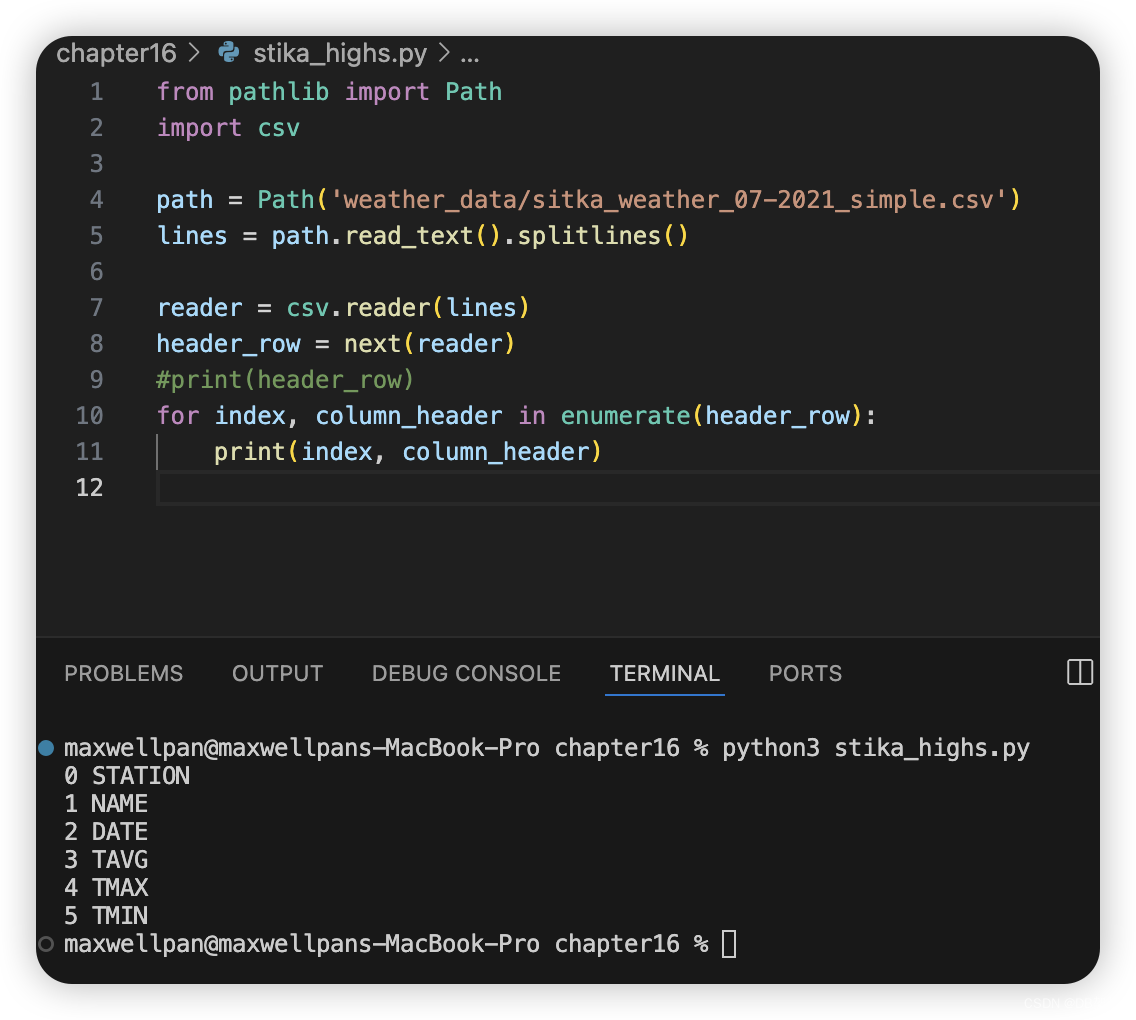
2.Parsing the CSV File Headers

from pathlib import Path
import csv

path = Path('weather_data/sitka_weather_07-2021_simple.csv')
lines = path.read_text().splitlines()

reader = csv.reader(lines)
header_row = next(reader)
print(header_row)

3. Printing the Headers and Their Positions

from pathlib import Path
import csv

path = Path('weather_data/sitka_weather_07-2021_simple.csv')
lines = path.read_text().splitlines()

reader = csv.reader(lines)
header_row = next(reader)
#print(header_row)
for index, column_header in enumerate(header_row):
    print(index, column_header)

4.Extracting and Reading Data

from pathlib import Path
import csv

path = Path('weather_data/sitka_weather_07-2021_simple.csv')
lines = path.read_text().splitlines()

reader = csv.reader(lines)
header_row = next(reader)

# Extract high temperatures.
highs = []
for row in reader:
    high = int(row[4])
    highs.append(high)

print(highs)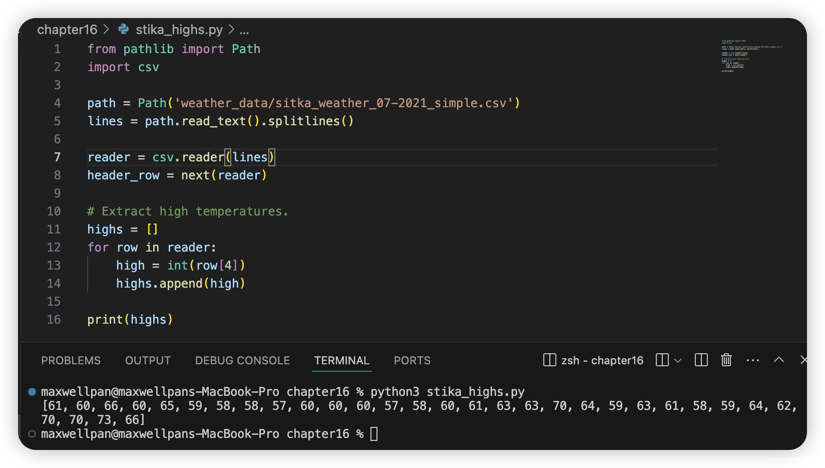

5.Plotting Data in a Temperature Chart

from pathlib import Path
import csv

import matplotlib.pyplot as plt

path = Path('weather_data/sitka_weather_07-2021_simple.csv')
lines = path.read_text().splitlines()

reader = csv.reader(lines)
header_row = next(reader)

# Extract high temperatures.
highs = []
for row in reader:
    high = int(row[4])
    highs.append(high)

print(highs)

# Plot the high temperatures.
plt.style.use('seaborn-v0_8')
fig, ax = plt.subplots()
ax.plot(highs, color='red')

# Format plot.
ax.set_title("Daily High Temperatures, July 2021", fontsize=24)
ax.set_xlabel('',fontsize=16)
ax.set_ylabel("Temperature(F)", fontsize=16)
ax.tick_params(labelsize=16)

plt.show()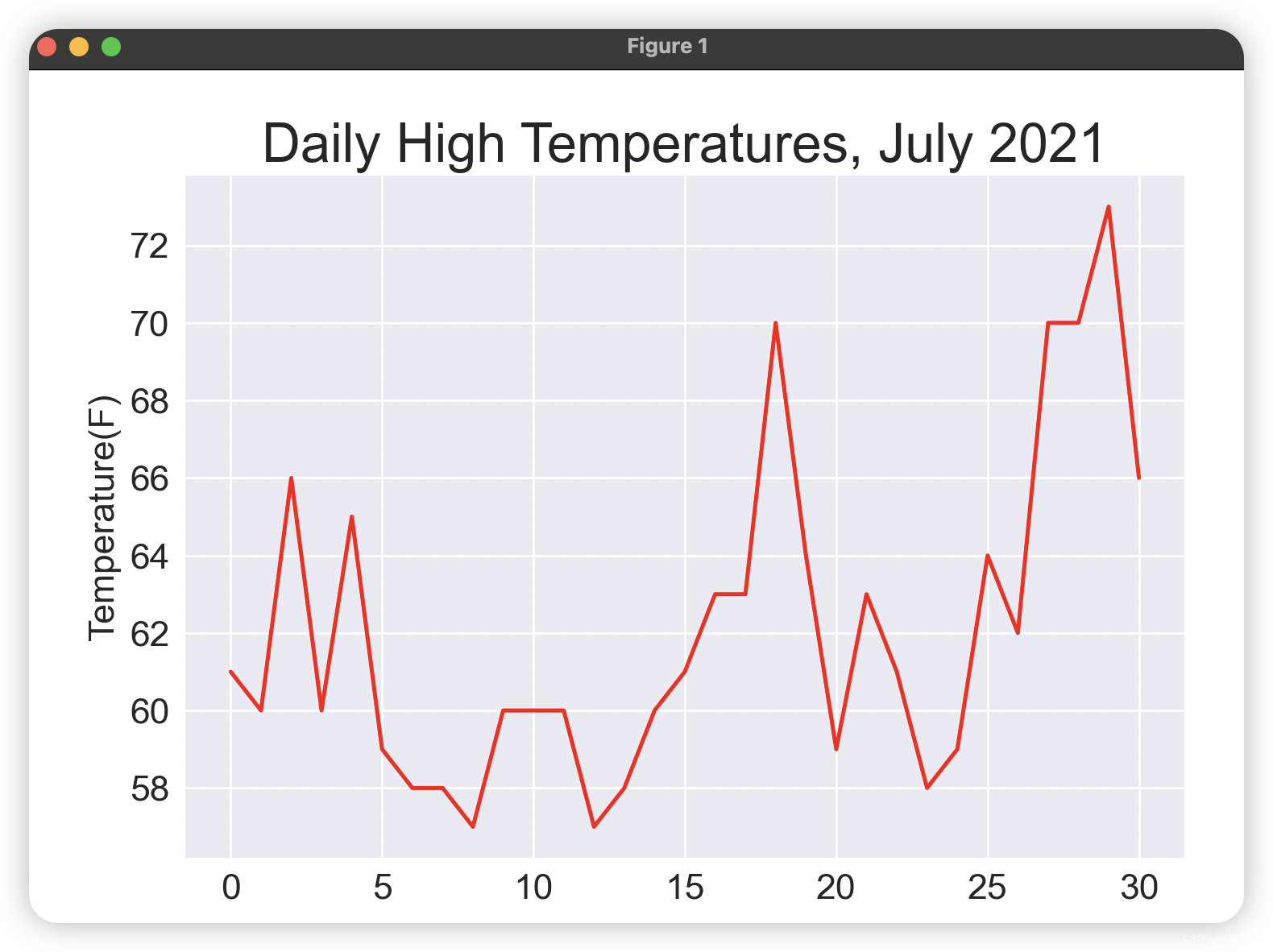

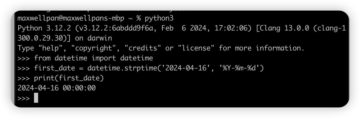
6.The datetime Module

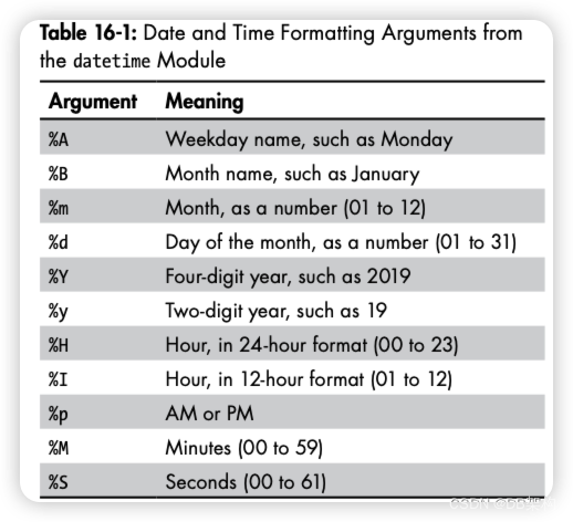
7.Plotting Dates

from pathlib import Path
import csv
from datetime import datetime

import matplotlib.pyplot as plt

path = Path('weather_data/sitka_weather_07-2021_simple.csv')
lines = path.read_text().splitlines()

reader = csv.reader(lines)
header_row = next(reader)

# Extract high temperatures.
dates, highs = [],[]
for row in reader:
    current_date = datetime.strptime(row[2], '%Y-%m-%d')
    high = int(row[4])
    dates.append(current_date)
    highs.append(high)

print(highs)

# Plot the high temperatures.
plt.style.use('seaborn-v0_8')
fig, ax = plt.subplots()
ax.plot(dates,highs, color='red')

# Format plot.
ax.set_title("Daily High Temperatures, July 2021", fontsize=24)
ax.set_xlabel('',fontsize=16)
fig.autofmt_xdate()
ax.set_ylabel("Temperature(F)", fontsize=16)
ax.tick_params(labelsize=16)

plt.show()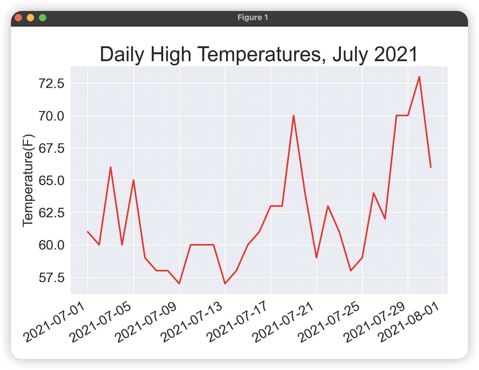

8.Plotting a Longer Timeframe

from pathlib import Path
import csv
from datetime import datetime

import matplotlib.pyplot as plt

path = Path('weather_data/sitka_weather_2021_simple.csv')
lines = path.read_text().splitlines()

reader = csv.reader(lines)
header_row = next(reader)

# Extract high temperatures.
dates, highs = [],[]
for row in reader:
    current_date = datetime.strptime(row[2], '%Y-%m-%d')
    high = int(row[4])
    dates.append(current_date)
    highs.append(high)

print(highs)

# Plot the high temperatures.
plt.style.use('seaborn-v0_8')
fig, ax = plt.subplots()
ax.plot(dates,highs, color='red')

# Format plot.
ax.set_title("Daily High Temperatures, 2021", fontsize=24)
ax.set_xlabel('',fontsize=16)
fig.autofmt_xdate()
ax.set_ylabel("Temperature(F)", fontsize=16)
ax.tick_params(labelsize=16)

plt.show()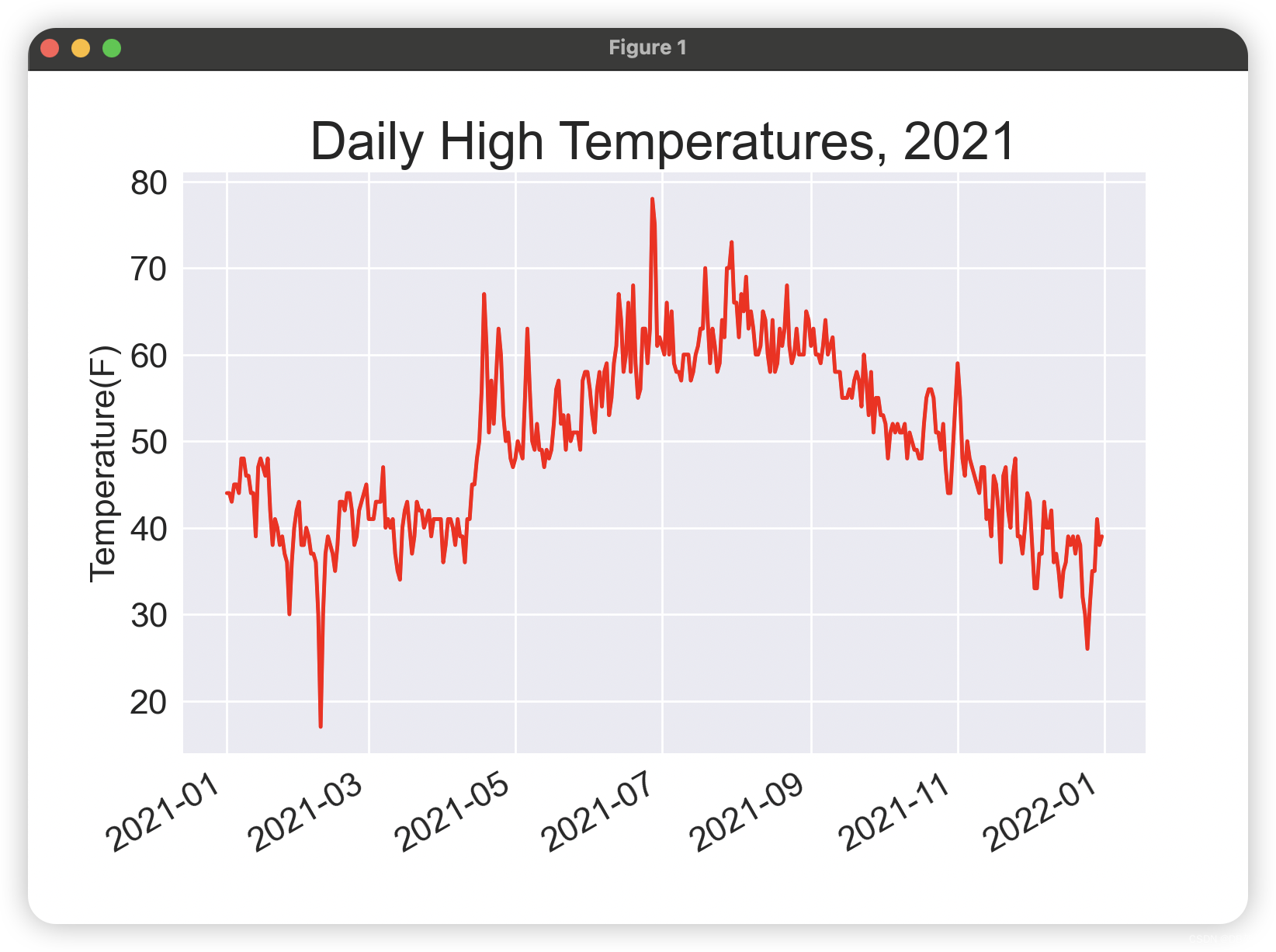

9.Plotting a Second Data Series

from pathlib import Path
import csv
from datetime import datetime

import matplotlib.pyplot as plt

path = Path('weather_data/sitka_weather_2021_simple.csv')
lines = path.read_text().splitlines()

reader = csv.reader(lines)
header_row = next(reader)

# Extract high temperatures.
dates, highs, lows = [],[],[]
for row in reader:
    current_date = datetime.strptime(row[2], '%Y-%m-%d')
    high = int(row[4])
    low = int(row[5])
    dates.append(current_date)
    highs.append(high)
    lows.append(low)


# Plot the high and low temperatures.
plt.style.use('seaborn-v0_8')
fig, ax = plt.subplots()
ax.plot(dates,highs, color='red')
ax.plot(dates, lows, color='blue')

# Format plot.
ax.set_title("Daily High and Low Temperatures, 2021", fontsize=24)
ax.set_xlabel('',fontsize=16)
fig.autofmt_xdate()
ax.set_ylabel("Temperature(F)", fontsize=16)
ax.tick_params(labelsize=16)

plt.show()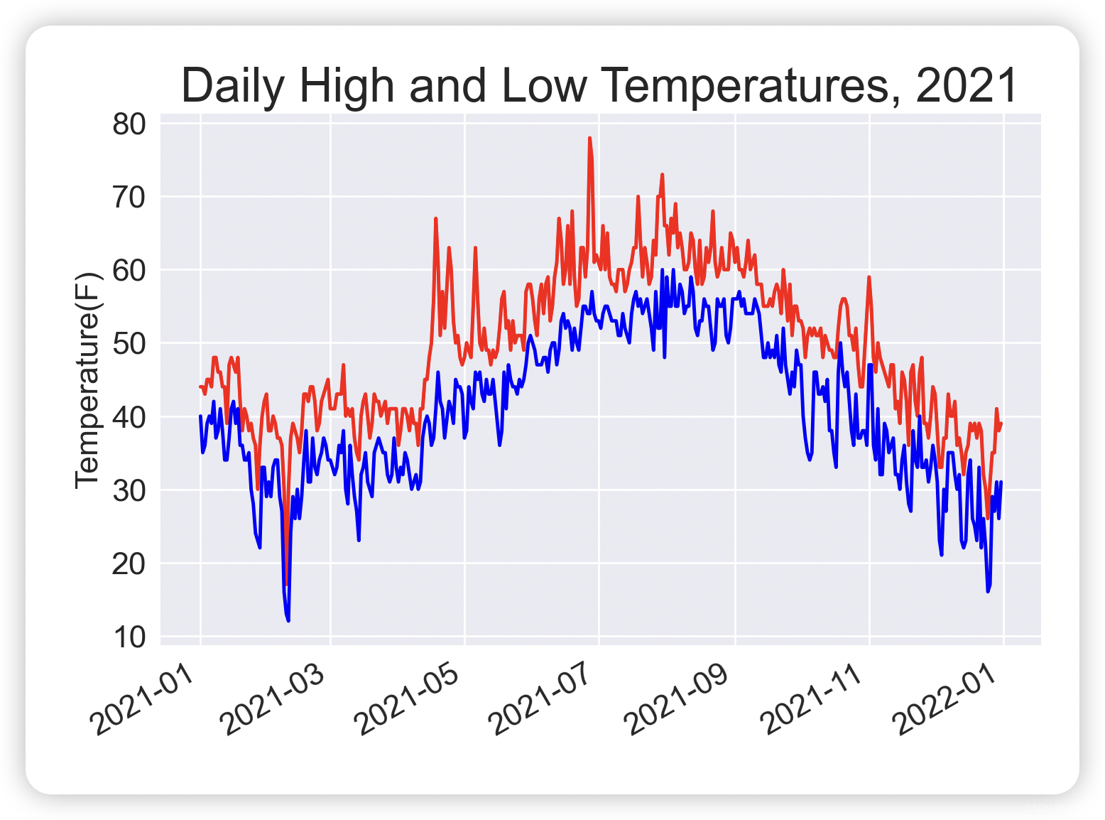

10.Shading an Area in the Chart

from pathlib import Path
import csv
from datetime import datetime

import matplotlib.pyplot as plt

path = Path('weather_data/sitka_weather_2021_simple.csv')
lines = path.read_text().splitlines()

reader = csv.reader(lines)
header_row = next(reader)

# Extract high temperatures.
dates, highs, lows = [],[],[]
for row in reader:
    current_date = datetime.strptime(row[2], '%Y-%m-%d')
    high = int(row[4])
    low = int(row[5])
    dates.append(current_date)
    highs.append(high)
    lows.append(low)


# Plot the high and low temperatures.
plt.style.use('seaborn-v0_8')
fig, ax = plt.subplots()
ax.plot(dates, highs, color='red', alpha=0.5)
ax.plot(dates, lows, color='blue', alpha=0.5)
ax.fill_between(dates, highs, lows, facecolor='blue', alpha=0.1)

# Format plot.
ax.set_title("Daily High and Low Temperatures, 2021", fontsize=24)
ax.set_xlabel('',fontsize=16)
fig.autofmt_xdate()
ax.set_ylabel("Temperature(F)", fontsize=16)
ax.tick_params(labelsize=16)

plt.show()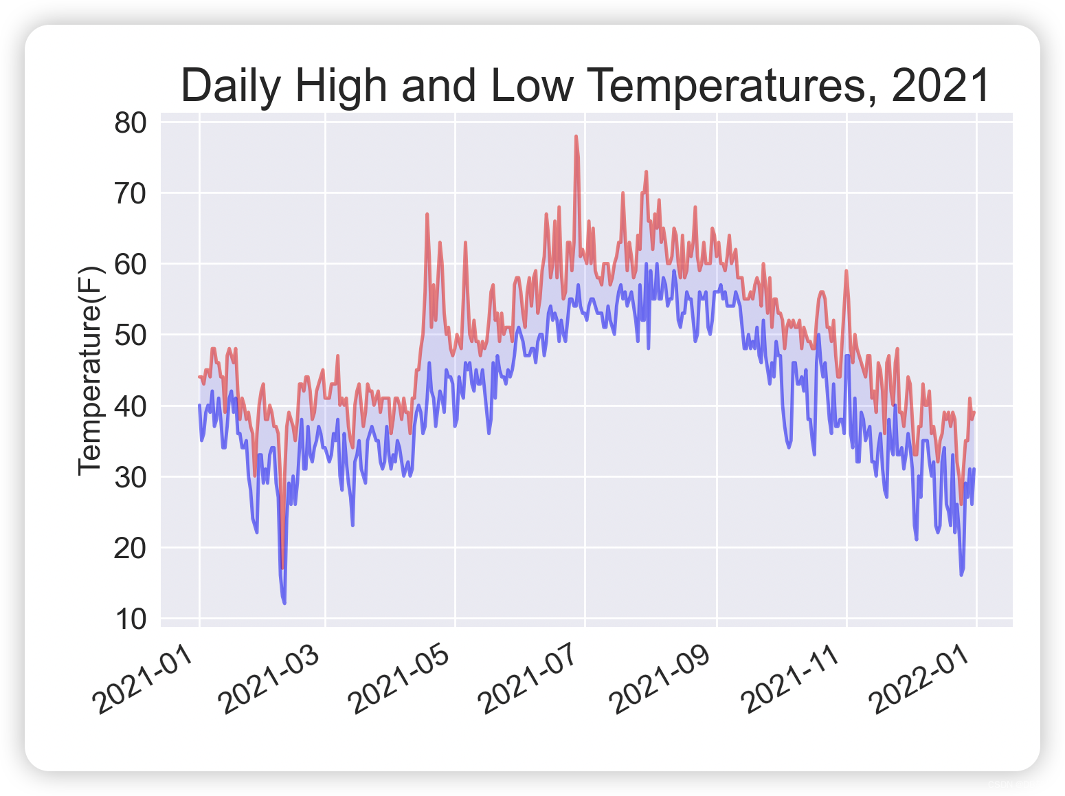

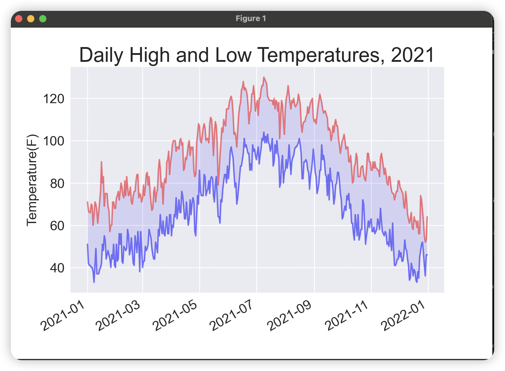
11.Error Checking

from pathlib import Path
import csv
from datetime import datetime
import matplotlib.pyplot as plt

path = Path('weather_data/death_valley_2021_simple.csv')
lines = path.read_text().splitlines()

reader = csv.reader(lines)
header_row = next(reader)

for index, column_header in enumerate(header_row):
    print(index, column_header)

# Extract dates, and high and low temperatures.
dates, highs, lows = [],[],[]
for row in reader:
    current_date = datetime.strptime(row[2], '%Y-%m-%d')
    try:
        high = int(row[3])
        low = int(row[4])
    except ValueError:
        print(f"Missing data for {current_date}")
    else:
        dates.append(current_date)
        highs.append(high)
        lows.append(low)

# Plot the high and low temperatures.
plt.style.use('seaborn-v0_8')
fig, ax = plt.subplots()
ax.plot(dates, highs, color='red', alpha=0.5)
ax.plot(dates, lows, color='blue', alpha=0.5)
ax.fill_between(dates, highs, lows, facecolor='blue', alpha=0.1)

# Format plot.
ax.set_title("Daily High and Low Temperatures, 2021", fontsize=24)
ax.set_xlabel('',fontsize=16)
fig.autofmt_xdate()
ax.set_ylabel("Temperature(F)", fontsize=16)
ax.tick_params(labelsize=16)

plt.show()

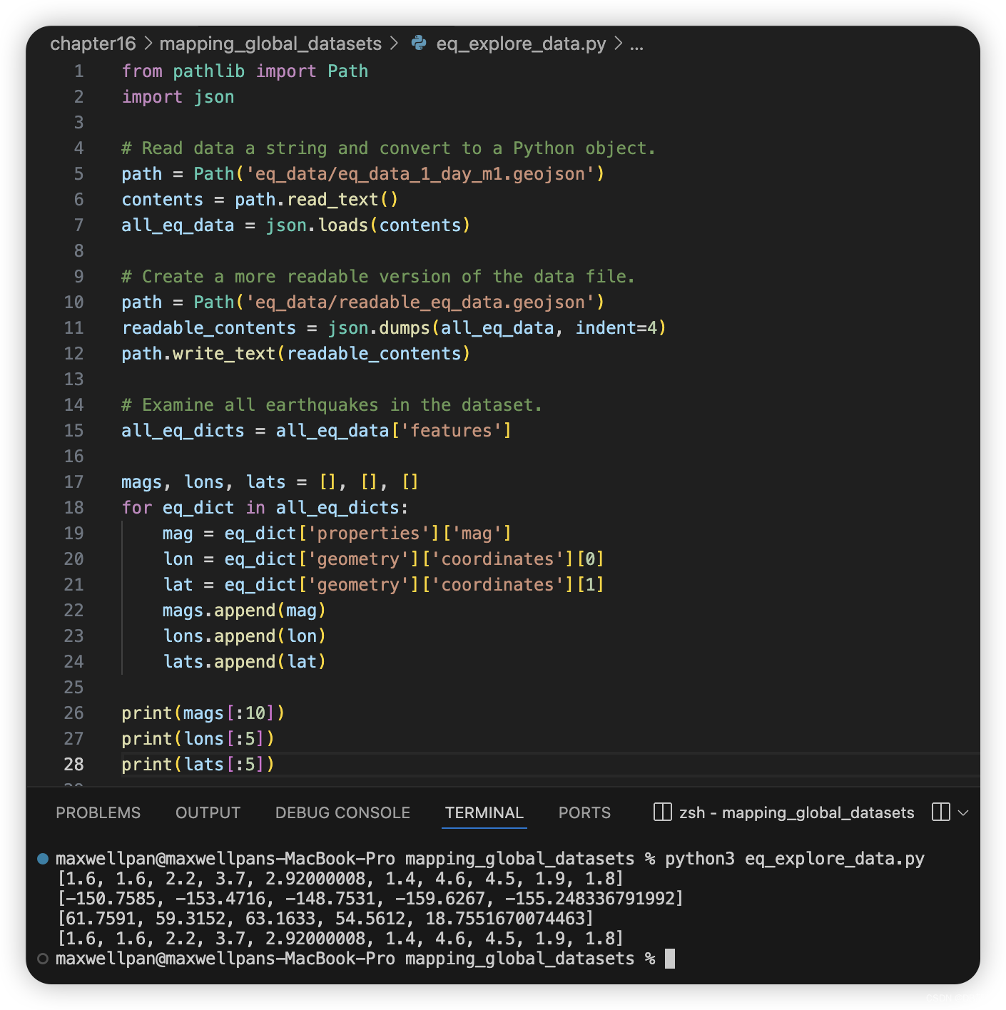
12. Mapping Global Datasets:GeoJSON Format

we read the data file as a string, and use json.loads() to convert the string representation of the file to a Python object. The json.dumps() can take an optional indent argument, which tells iit how much to indent nested elements in the data structure.

from pathlib import Path
import json

# Read data a string and convert to a Python object.
path = Path('eq_data/eq_data_1_day_m1.geojson')
contents = path.read_text()
all_eq_data = json.loads(contents)

# Create a more readable version of the data file.
path = Path('eq_data/readable_eq_data.geojson')
readable_contents = json.dumps(all_eq_data, indent=4)
path.write_text(readable_contents)

13. Making a List of All Earthquakes

from pathlib import Path
import json

# Read data a string and convert to a Python object.
path = Path('eq_data/eq_data_1_day_m1.geojson')
contents = path.read_text()
all_eq_data = json.loads(contents)

# Create a more readable version of the data file.
path = Path('eq_data/readable_eq_data.geojson')
readable_contents = json.dumps(all_eq_data, indent=4)
path.write_text(readable_contents)

# Examine all earthquakes in the dataset.
all_eq_dicts = all_eq_data['features']
print(len(all_eq_dicts))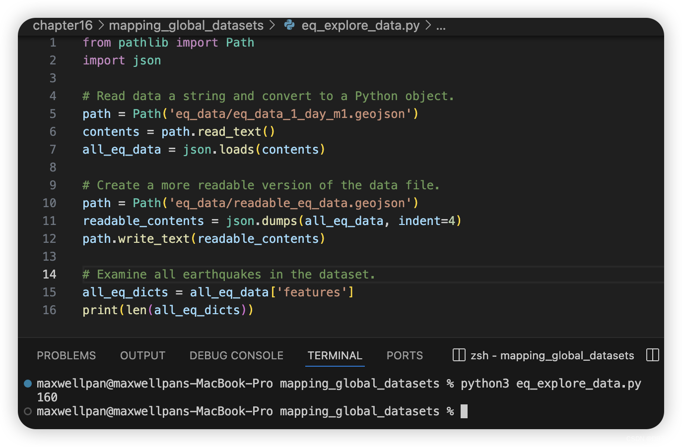

 14. Extracting Magnitudes

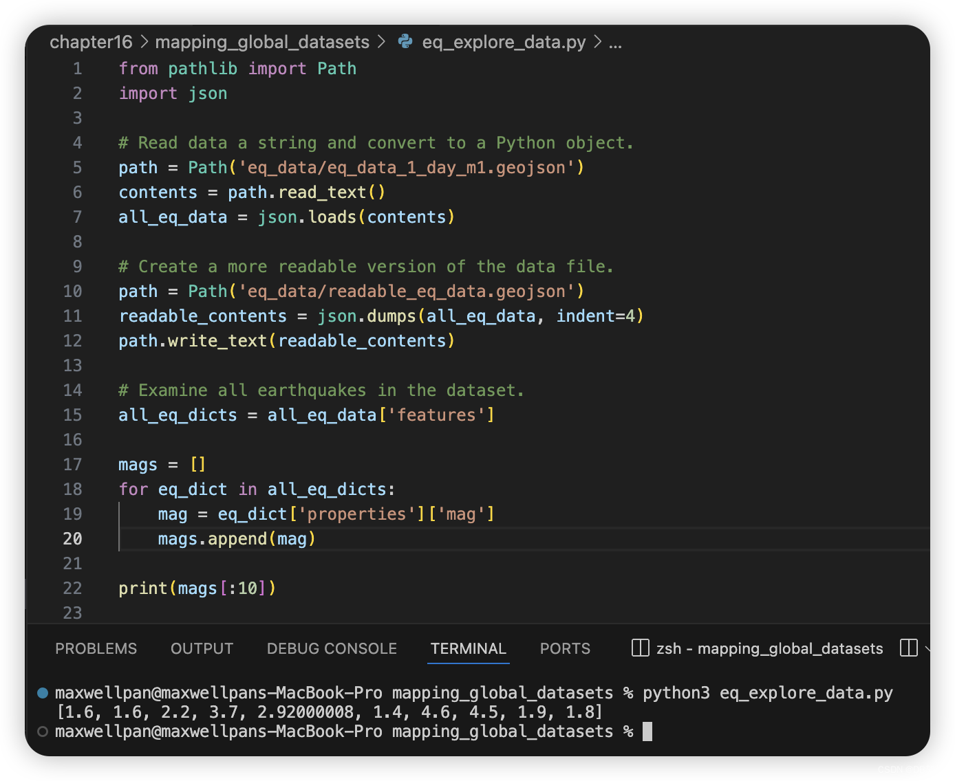
from pathlib import Path
import json

# Read data a string and convert to a Python object.
path = Path('eq_data/eq_data_1_day_m1.geojson')
contents = path.read_text()
all_eq_data = json.loads(contents)

# Create a more readable version of the data file.
path = Path('eq_data/readable_eq_data.geojson')
readable_contents = json.dumps(all_eq_data, indent=4)
path.write_text(readable_contents)

# Examine all earthquakes in the dataset.
all_eq_dicts = all_eq_data['features']

mags = []
for eq_dict in all_eq_dicts:
    mag = eq_dict['properties']['mag']
    mags.append(mag)

print(mags[:10])

 15.Extracting Location Data

from pathlib import Path
import json

# Read data a string and convert to a Python object.
path = Path('eq_data/eq_data_1_day_m1.geojson')
contents = path.read_text()
all_eq_data = json.loads(contents)

# Create a more readable version of the data file.
path = Path('eq_data/readable_eq_data.geojson')
readable_contents = json.dumps(all_eq_data, indent=4)
path.write_text(readable_contents)

# Examine all earthquakes in the dataset.
all_eq_dicts = all_eq_data['features']

mags, lons, lats = [], [], []
for eq_dict in all_eq_dicts:
    mag = eq_dict['properties']['mag']
    lon = eq_dict['geometry']['coordinates'][0]
    lat = eq_dict['geometry']['coordinates'][1]
    mags.append(mag)
    lons.append(lon)
    lats.append(lat)

print(mags[:10])
print(lons[:5])
print(lats[:5])

print(mags[:10])

16.Building a World Map

from pathlib import Path
import json

import plotly.express as px

# Read data a string and convert to a Python object.
path = Path('eq_data/eq_data_1_day_m1.geojson')
contents = path.read_text()
all_eq_data = json.loads(contents)

# Create a more readable version of the data file.
path = Path('eq_data/readable_eq_data.geojson')
readable_contents = json.dumps(all_eq_data, indent=4)
path.write_text(readable_contents)

# Examine all earthquakes in the dataset.
all_eq_dicts = all_eq_data['features']

mags, lons, lats = [], [], []
for eq_dict in all_eq_dicts:
    mag = eq_dict['properties']['mag']
    lon = eq_dict['geometry']['coordinates'][0]
    lat = eq_dict['geometry']['coordinates'][1]
    mags.append(mag)
    lons.append(lon)
    lats.append(lat)

print(mags[:10])
print(lons[:5])
print(lats[:5])

print(mags[:10])

title = 'Global Earthquakes'
fig = px.scatter_geo(lat=lats, lon=lons, title=title)
fig.show()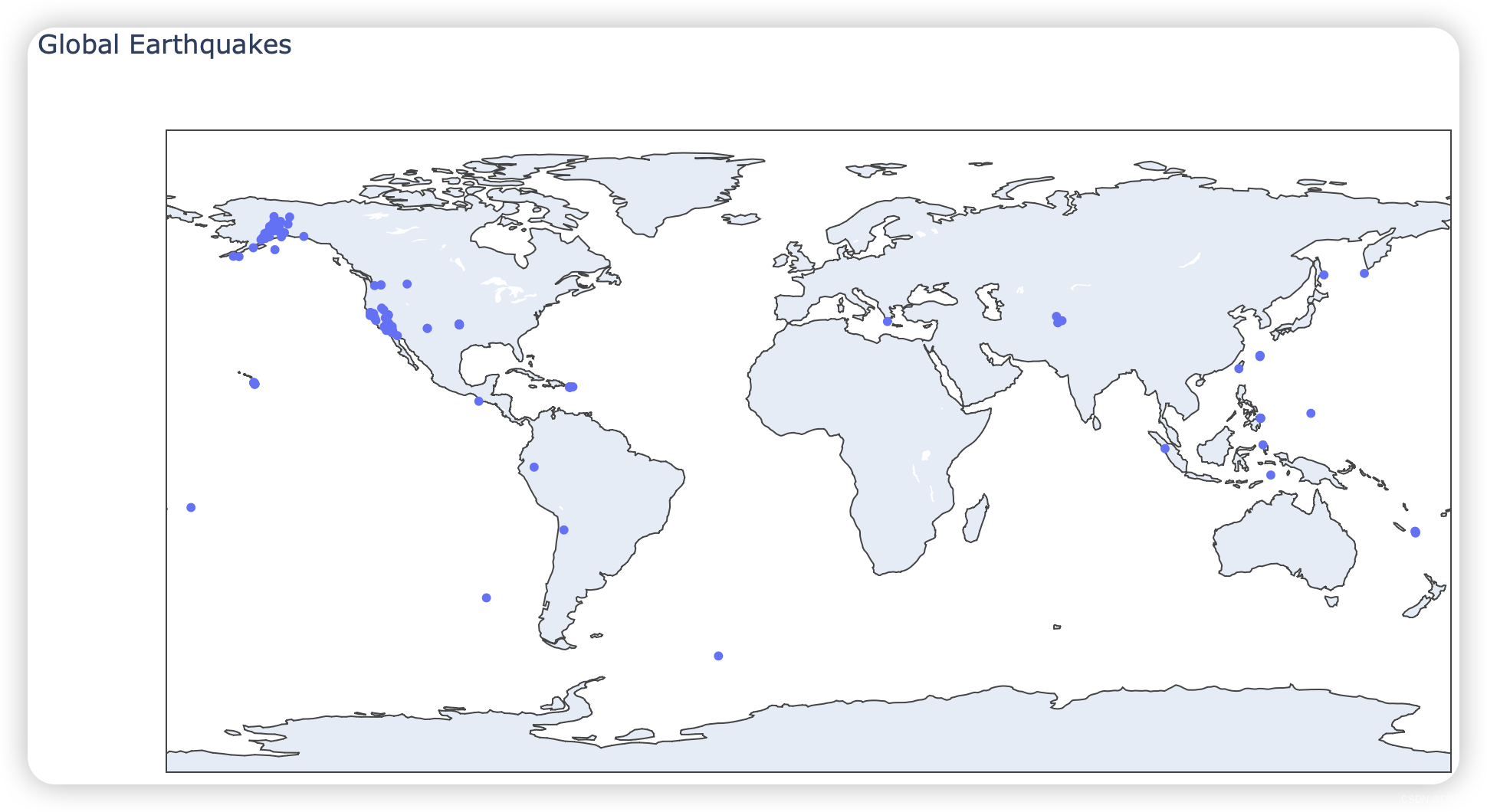

17. Representing Magnitudes

from pathlib import Path
import json

import plotly.express as px

# Read data a string and convert to a Python object.
path = Path('eq_data/eq_data_30_day_m1.geojson')
contents = path.read_text()
all_eq_data = json.loads(contents)

# Create a more readable version of the data file.
path = Path('eq_data/readable_eq_data.geojson')
readable_contents = json.dumps(all_eq_data, indent=4)
path.write_text(readable_contents)

# Examine all earthquakes in the dataset.
all_eq_dicts = all_eq_data['features']

mags, lons, lats = [], [], []
for eq_dict in all_eq_dicts:
    mag = eq_dict['properties']['mag']
    lon = eq_dict['geometry']['coordinates'][0]
    lat = eq_dict['geometry']['coordinates'][1]
    mags.append(mag)
    lons.append(lon)
    lats.append(lat)

print(mags[:10])
print(lons[:5])
print(lats[:5])

print(mags[:10])

title = 'Global Earthquakes'
fig = px.scatter_geo(lat=lats, lon=lons, size=mags, title=title)
fig.show()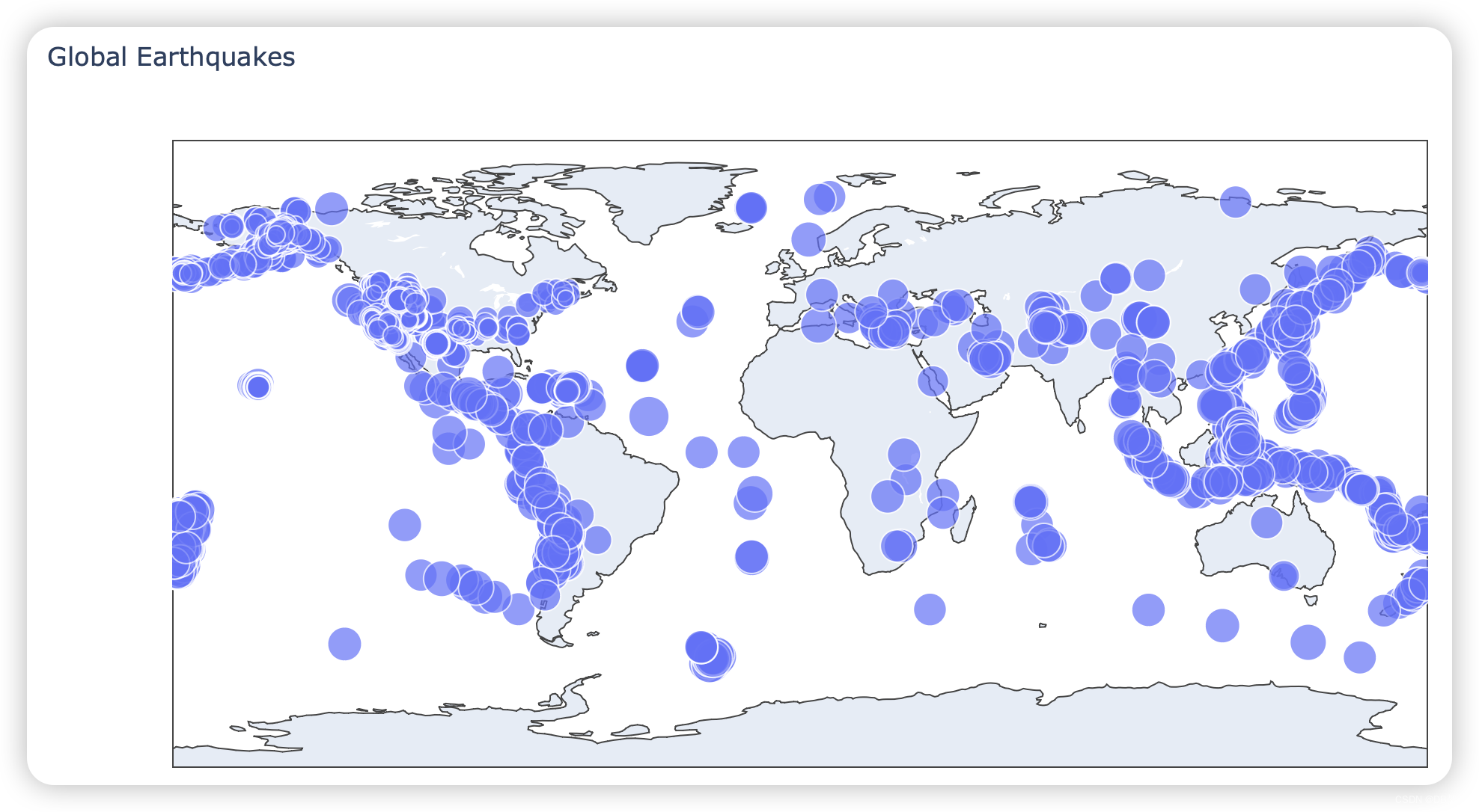

 18. Customing Marker Colors

from pathlib import Path
import json

import plotly.express as px

# Read data a string and convert to a Python object.
path = Path('eq_data/eq_data_30_day_m1.geojson')
contents = path.read_text()
all_eq_data = json.loads(contents)

# Create a more readable version of the data file.
path = Path('eq_data/readable_eq_data.geojson')
readable_contents = json.dumps(all_eq_data, indent=4)
path.write_text(readable_contents)

# Examine all earthquakes in the dataset.
all_eq_dicts = all_eq_data['features']

mags, lons, lats = [], [], []
for eq_dict in all_eq_dicts:
    mag = eq_dict['properties']['mag']
    lon = eq_dict['geometry']['coordinates'][0]
    lat = eq_dict['geometry']['coordinates'][1]
    mags.append(mag)
    lons.append(lon)
    lats.append(lat)

print(mags[:10])
print(lons[:5])
print(lats[:5])

print(mags[:10])

title = 'Global Earthquakes'
fig = px.scatter_geo(lat=lats, lon=lons, size=mags, title=title,
                     color=mags,
                     color_continuous_scale='Viridis',
                     labels={'color':'Magnitude'},
                     projection='natural earth',)
fig.show()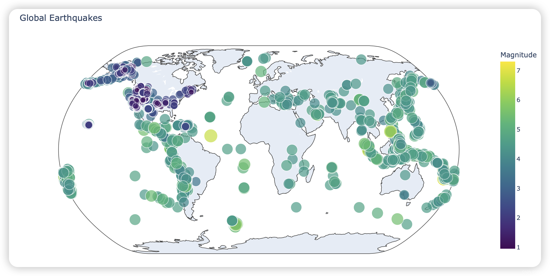

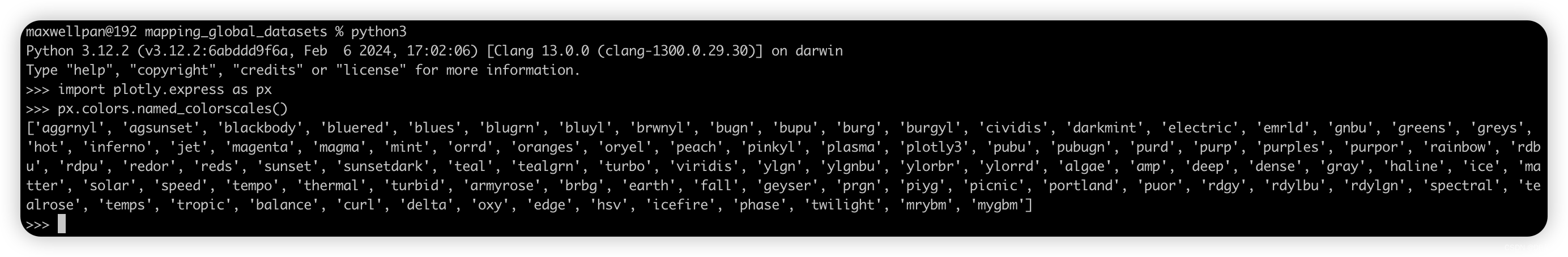
19.Other Color Scales

maxwellpan@192 mapping_global_datasets % python3
Python 3.12.2 (v3.12.2:6abddd9f6a, Feb  6 2024, 17:02:06) [Clang 13.0.0 (clang-1300.0.29.30)] on darwin
Type "help", "copyright", "credits" or "license" for more information.
>>> import plotly.express as px
>>> px.colors.named_colorscales()
['aggrnyl', 'agsunset', 'blackbody', 'bluered', 'blues', 'blugrn', 'bluyl', 'brwnyl', 'bugn', 'bupu', 'burg', 'burgyl', 'cividis', 'darkmint', 'electric', 'emrld', 'gnbu', 'greens', 'greys', 'hot', 'inferno', 'jet', 'magenta', 'magma', 'mint', 'orrd', 'oranges', 'oryel', 'peach', 'pinkyl', 'plasma', 'plotly3', 'pubu', 'pubugn', 'purd', 'purp', 'purples', 'purpor', 'rainbow', 'rdbu', 'rdpu', 'redor', 'reds', 'sunset', 'sunsetdark', 'teal', 'tealgrn', 'turbo', 'viridis', 'ylgn', 'ylgnbu', 'ylorbr', 'ylorrd', 'algae', 'amp', 'deep', 'dense', 'gray', 'haline', 'ice', 'matter', 'solar', 'speed', 'tempo', 'thermal', 'turbid', 'armyrose', 'brbg', 'earth', 'fall', 'geyser', 'prgn', 'piyg', 'picnic', 'portland', 'puor', 'rdgy', 'rdylbu', 'rdylgn', 'spectral', 'tealrose', 'temps', 'tropic', 'balance', 'curl', 'delta', 'oxy', 'edge', 'hsv', 'icefire', 'phase', 'twilight', 'mrybm', 'mygbm']
>>>

 20.Adding Hover Text

from pathlib import Path
import json

import plotly.express as px

# Read data a string and convert to a Python object.
path = Path('eq_data/eq_data_30_day_m1.geojson')
contents = path.read_text()
all_eq_data = json.loads(contents)

# Create a more readable version of the data file.
path = Path('eq_data/readable_eq_data.geojson')
readable_contents = json.dumps(all_eq_data, indent=4)
path.write_text(readable_contents)

# Examine all earthquakes in the dataset.
all_eq_dicts = all_eq_data['features']

mags, lons, lats, eq_titles = [], [], [], []
for eq_dict in all_eq_dicts:
    mag = eq_dict['properties']['mag']
    lon = eq_dict['geometry']['coordinates'][0]
    lat = eq_dict['geometry']['coordinates'][1]
    eq_title = eq_dict['properties']['title']
    mags.append(mag)
    lons.append(lon)
    lats.append(lat)
    eq_titles.append(eq_title)

print(mags[:10])
print(lons[:5])
print(lats[:5])

print(mags[:10])

title = 'Global Earthquakes'
fig = px.scatter_geo(lat=lats, lon=lons, size=mags, title=title,
                     color=mags,
                     color_continuous_scale='Viridis',
                     labels={'color':'Magnitude'},
                     projection='natural earth',
                     hover_name=eq_titles,)
fig.show()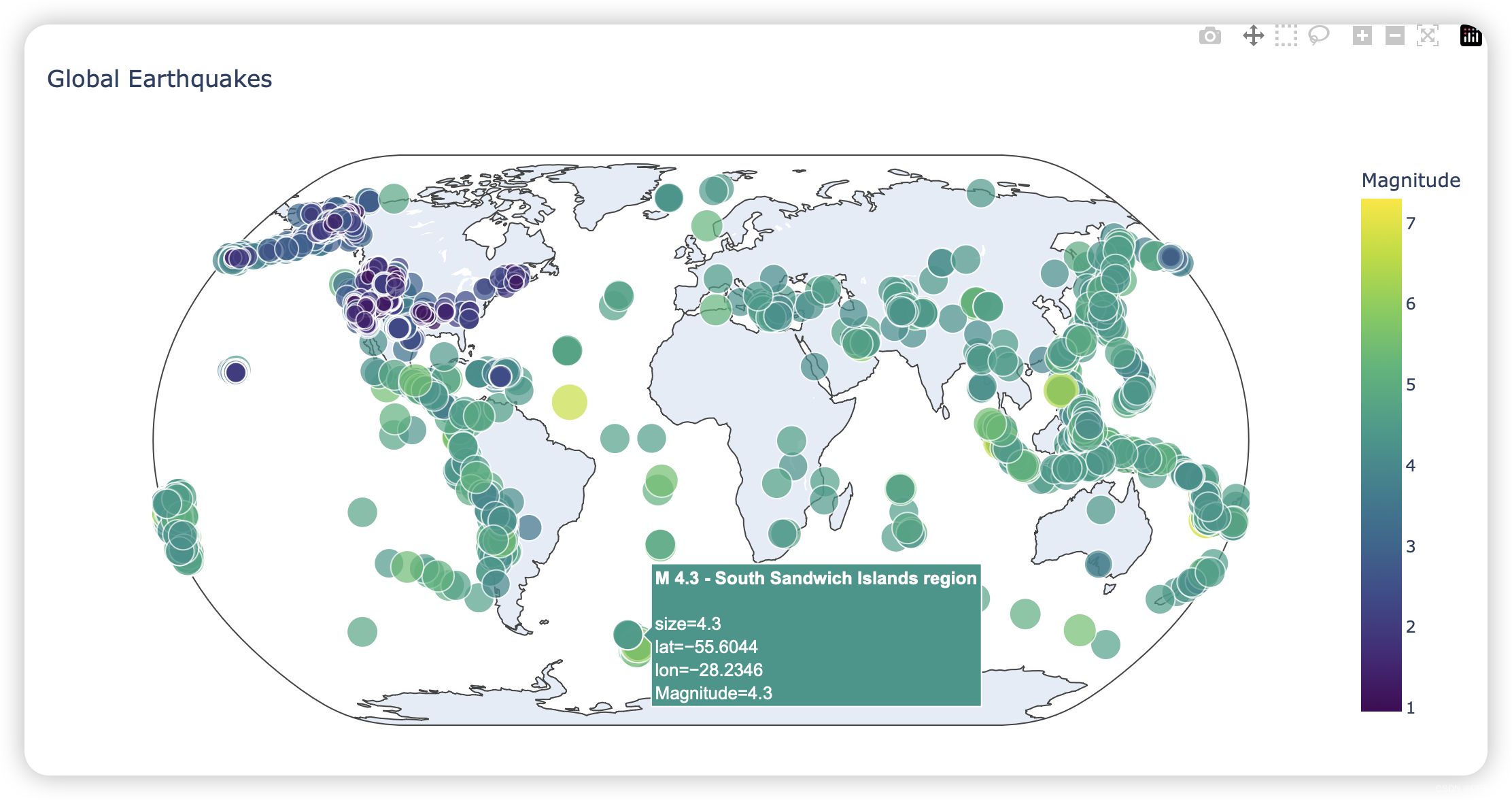

 21.Summary

we learned how to work with real-world datasets.Ypi processed CSV and GeoJSON files, and extracted the data you want to focus on. Using historical weather data, we learned more about working with Matplotlib, including how to use the datetime module and how to plot multiple data series on one chart. We plotted geographical data on a world map in Plotly, and learned to cusotmize the style of the map.

22.Sharing

pcc_3e/chapter_16 at main · psmaxwell/pcc_3e · GitHub