


 本文探讨了VC维的概念,即假设集在数据集上所能达到的最大分类情况,揭示了其与模型复杂度的关系。通过解析感知器的VC维,阐述了模型复杂度对样本需求的影响,以及VC维在理论与实践中的差异。
Lecture 7: The VC Dimension
Definition of VC Dimension
m H ( N ) m_{\mathcal{H}}(N) mH(N) breaks at k(good H H H) and N large enough(good D D D) => E o u t ≈ E i n E_{\mathrm{out}} \approx E_{\mathrm{in}} Eout≈Ein
A A A picks a g g g with small E i n E_{in} Ein (good A A A) => E i n ≈ 0 E_{\mathrm{in}} \approx 0 Ein≈0
最后学到了东西,到达了要求 => E o u t ≈ 0 E_{\mathrm{out}} \approx 0 Eout≈0
VC Dimension
VC Dimension is the maximum of non-break point.
largest N for which
m
H
(
N
)
m_H (N)
mH(N) =
2
N
2^N
2N
d
v
c
d_{vc}
dvc = ‘minimum k’ - 1
the most inputs
H
H
H that can shatter
VC Dimension反映了假设集在数据集上的性质:数据集的最大分类情况。
d
v
c
d_{vc}
dvc和minimum break point都是"一线曙光"的分界点。
i
f
N
≥
2
,
d
v
c
≥
2
,
m
H
(
N
)
≤
N
d
v
c
if \ N \geq 2, d_{\mathrm{vc}} \geq 2, m_{\mathcal{H}}(N) \leq N^{d_{\mathrm{vc}}}
if N≥2,dvc≥2,mH(N)≤Ndvc
和之前一样(minimum break point finite),我们希望 d v c d_{vc} dvc finite.
Fun Time
If there is a set of
N
N
N inputs that cannot be shattered by
H
H
H. Based only on this information, what can we conclude about
d
V
C
(
H
)
d_{VC} (H)
dVC(H)?
1
d
v
c
(
H
)
>
N
d_{\mathrm{vc}}(\mathcal{H})>N
dvc(H)>N
2
d
v
c
(
H
)
=
N
d_{\mathrm{vc}}(\mathcal{H})=N
dvc(H)=N
3
d
v
c
(
H
)
<
N
d_{\mathrm{vc}}(\mathcal{H})<N
dvc(H)<N
4 no conclusion can be made
✓
\checkmark
✓
Explanation
这道题目当初也是百思不得其解,直到我又学习了一遍。
VC Dimension:the most inputs
H
H
H that can shatter
有N个数据no shatter不能代表其他的N个数据no shatter。
举例说明:
1维感知器 break point为3, 2维感知器 break point为4。
在2维空间中,连成一条直线的三个点(2维退化到1维),分类数只有6(
<
2
3
<2^3
<23)种 。而2维感知器的break point却为4,这就是因为不在同一条直线上的三个点分类数可以为8。所以导致2维感知器的最小break point增大了。
这里面也蕴含着提升维度,增大了自由度。?
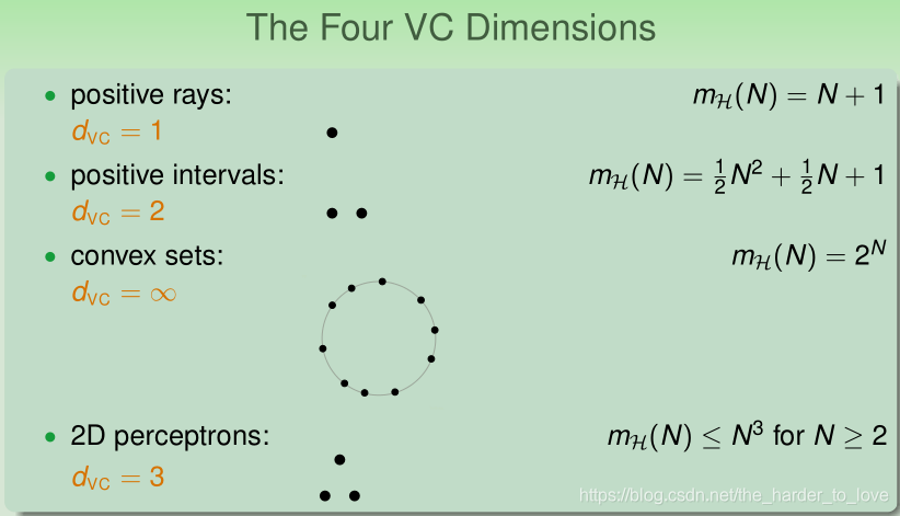
VC Dimension of Perceptrons
1D perceptron (pos/neg rays):
d
v
c
d_{\mathrm{vc}}
dvc = 2
2D perceptrons:
d
v
c
d_{\mathrm{vc}}
dvc = 3
d-D perceptrons:
d
v
c
=
d
+
1
d_{\mathrm{vc}}= d + 1
dvc=d+1
证明分两步:
•
d
v
c
≥
d
+
1
d_{\mathrm{vc}}≥ d + 1
dvc≥d+1:存在(d+1)个点 shatter.
•
d
v
c
≤
d
+
1
d_{\mathrm{vc}} ≤ d + 1
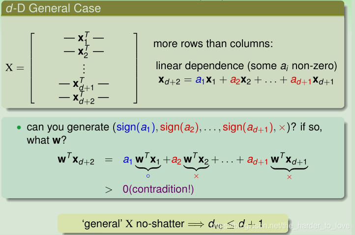
dvc≤d+1:任何(d+2)个点 no shatter.
Extra Fun Time
What statement below shows that
d
v
c
≥
d
+
1
d_{\mathrm{vc}}≥ d + 1
dvc≥d+1
1 There are some d + 1 inputs we can shatter.
✓
\checkmark
✓
2 We can shatter any set of d + 1 inputs.
3 There are some d + 2 inputs we cannot shatter.
4 We cannot shatter any set of d + 2 inputs.
Explanation
存在(d+1)个点 shatter =>
d
v
c
≥
d
+
1
d_{\mathrm{vc}}≥ d + 1
dvc≥d+1
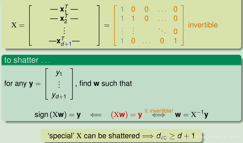
Special X(d+1个点) 对于任意的y,都有对应的hypothesis(w) .
Extra Fun Time
What statement below shows that
d
v
c
≤
d
+
1
d_{\mathrm{vc}} \le d + 1
dvc≤d+1
1 There are some d + 1 inputs we can shatter.
2 We can shatter any set of d + 1 inputs.
3 There are some d + 2 inputs we cannot shatter.
4 We cannot shatter any set of d + 2 inputs.
✓
\checkmark
✓
Explanation
任何(d+2)个点 no shatter. =>
d
v
c
≤
d
+
1
d_{\mathrm{vc}} ≤ d + 1
dvc≤d+1
x
d
+
2
x_{d+2}
xd+2与
x
1
,
x
2
,
.
.
.
,
x
d
+
1
x_1,x_2,...,x_{d+1}
x1,x2,...,xd+1线性相关,假设这任意d+2个点可以shatter,那么
a
1
,
a
2
,
.
.
.
,
a
d
+
1
,
a
d
+
2
a_1,a_2,...,a_{d+1},a_{d+2}
a1,a2,...,ad+1,ad+2系数可以任意取,当
a
i
=
s
i
g
n
(
w
T
x
i
)
a_i=sign(w^Tx_i)
ai=sign(wTxi)时,
w
T
x
d
>
0
w^Tx_d>0
wTxd>0,所以d+2个点no shatter.
Fun Time
Based on the proof above, what is d VC of 1126-D perceptrons?
1 1024
2 1126
3 1127
✓
\checkmark
✓
4 6211
Explanation
d-D perceptrons:
d
v
c
=
d
+
1
d_{\mathrm{vc}}= d + 1
dvc=d+1
Physical Intuition of VC Dimension
d
v
c
(
H
)
d_{\mathrm{vc}}(H)
dvc(H): powerfulness of
H
H
H
d
v
c
d_{\mathrm{vc}}
dvc ≈ #free parameters
d
v
c
d_{\mathrm{vc}}
dvc代表了自由度(与自由变量的个数相关),我在学统计学时接触过自由度这个概念,若
μ
\mu
μ(均值)确定,数据大小为N的自由度就为N-1,因为
μ
\mu
μ确定,知道N-1个点,就能求出第N个点。
d
V
C
(
H
)
d_{VC}(H)
dVC(H)就代表了
H
H
H关于数据的自由度。
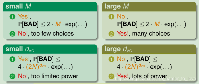
M and d V C d_{VC} dVC
so choose the right
h
y
p
o
t
h
e
s
i
s
s
e
t
hypothesis \ set
hypothesis set(
M
M
M or
d
v
c
d_{\mathrm{vc}}
dvc).
Fun Time
Origin-crossing Hyperplanes are essentially perceptrons with
w
0
w_0
w0 fixed at 0. Make a guess about the
d
v
c
d_{\mathrm{vc}}
dvc of origin-crossing hyperplanes in
R
d
R_d
Rd.
1 1
2 d
✓
\checkmark
✓
3 d+1
4
∞
\infty
∞
Explanation
d-D perceptrons:
d
v
c
=
d
+
1
d_{\mathrm{vc}}= d + 1
dvc=d+1
而穿过原点,加了一个限制条件,使自由度降1,故变成了d.
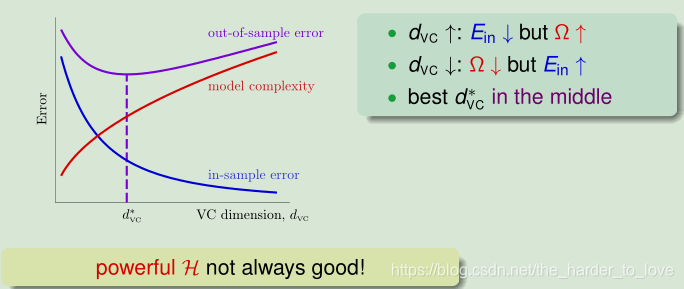
Interpreting VC Dimension
Penalty for Model Complexity
P D [ [ E in ( g ) − E out ( g ) ∣ > ϵ ] ⎵ BAD ] ≤ 4 ( 2 N ) d v c exp ( − 1 8 ϵ 2 N ) ⎵ δ p r o b a b i l i t y ≥ 1 − δ , GOOD : ∣ E i n ( g ) − E o u t ( g ) ∣ ≤ ϵ δ = 4 ( 2 N ) d v c exp ( − 1 8 ϵ 2 N ) ϵ = 8 N ln ( 4 ( 2 N ) d v c δ ) E i n ( g ) − 8 N ln ( 4 ( 2 N ) d v c δ ) ≤ E o u t ( g ) ≤ E i n ( g ) + 8 N ln ( 4 ( 2 N ) d v c δ ) 8 N ln ( 4 ( 2 N ) d v c δ ) ⎵ Ω ( N , H , δ ) penalty for model complexity \mathbb{P}_{\mathcal{D}}\left[\underbrace{\left[E_{\text { in }}(g)-E_{\text { out }}(g) |>\epsilon\right]}_{\text { BAD }}\right] \leq \underbrace{4(2 N)^{d_{vc}} \exp \left(-\frac{1}{8} \epsilon^{2} N\right)}_{\delta} \\ probability ≥ 1 − \delta, \ \operatorname{GOOD} : | E_{in}(g)-E_{out}(g) | \leq \epsilon \\ \delta=4(2 N)^{d_{\mathrm{vc}}} \exp \left(-\frac{1}{8} \epsilon^{2} N\right) \\ \epsilon = \sqrt{\frac{8}{N} \ln \left(\frac{4(2 N)^{d_{\mathrm{vc}}}}{\delta}\right)} \\ E_{in}(g) - \sqrt{\frac{8}{N} \ln \left(\frac{4(2 N)^{d_{\mathrm{vc}}}}{\delta}\right)} \leq E_{out}(g) \leq E_{in}(g) + \sqrt{\frac{8}{N} \ln \left(\frac{4(2 N)^{d_{\mathrm{vc}}}}{\delta}\right)} \\ \underbrace{\sqrt{\frac{8}{N} \ln \left(\frac{4(2 N)^{d_{\mathrm{vc}}}}{\delta}\right)}}_{\Omega(N, \mathcal{H}, \delta)} \quad \text{ penalty for model complexity} PD⎣⎡ BAD [E in (g)−E out (g)∣>ϵ]⎦⎤≤δ 4(2N)dvcexp(−81ϵ2N)probability≥1−δ, GOOD:∣Ein(g)−Eout(g)∣≤ϵδ=4(2N)dvcexp(−81ϵ2N)ϵ=N8ln(δ4(2N)dvc)Ein(g)−N8ln(δ4(2N)dvc)≤Eout(g)≤Ein(g)+N8ln(δ4(2N)dvc)Ω(N,H,δ) N8ln(δ4(2N)dvc) penalty for model complexity
Sample Complexity
P D [ ∣ E in ( g ) − E out ( g ) ∣ > ϵ ⎵ BAD ] ≤ 4 ( 2 N ) d 0 exp ( − 1 8 ϵ 2 N ) ⎵ δ given ϵ = 0.1 , δ = 0.1 , d v c = 3 N bound 100 2.82 × 1 0 7 1 , 000 9.17 × 1 0 9 10 , 000 1.19 × 1 0 8 100 , 000 1.65 × 1 0 − 38 29 , 300 9.99 × 1 0 − 2 sample complexity: N ≈ 10 , 000 d v c in theory \mathbb{P}_{\mathcal{D}}\left[\underbrace{ | E_{\text { in }}(g)-E_{\text { out }}(g) |>\epsilon}_{\text { BAD }}\right] \leq \underbrace{4(2 N)^{d_{0}} \exp \left(-\frac{1}{8} \epsilon^{2} N\right)}_{\delta} ~\\ ~\\ ~\\ \\ \text{given} \ \epsilon=0.1, \delta=0.1, d_{\mathrm{vc}}=3 ~\\ ~\\ \begin{array}{cc}{N} & {\text { bound }} \\ {100} & {2.82 \times 10^{7}} \\ {1,000} & {9.17 \times 10^{9}} \\ {10,000} & {1.19 \times 10^{8}} \\ {100,000} & {1.65 \times 10^{-38}} \\ {29,300} & {9.99 \times 10^{-2}}\end{array} \\ \text{sample complexity:} \ N \approx 10,000 d_{\mathrm{vc}} \text{in theory} PD⎣⎡ BAD ∣E in (g)−E out (g)∣>ϵ⎦⎤≤δ 4(2N)d0exp(−81ϵ2N) given ϵ=0.1,δ=0.1,dvc=3 N1001,00010,000100,00029,300 bound 2.82×1079.17×1091.19×1081.65×10−389.99×10⁻²sample complexity: N≈10,000dvcin theory
import math


# 计算VC Bound
def count_vc_bound(N, epsilon=0.1, delta=0.1, d_vc=3):
    vc_bound = 4*(2*N)**d_vc*math.exp(-0.125*epsilon**2*N)
    return vc_bound


if __name__ == '__main__':
    print('%e' % count_vc_bound(100))
    print('%e' % count_vc_bound(1000))
    print('%e' % count_vc_bound(10000))
    print('%e' % count_vc_bound(100000))
    print('%e' % count_vc_bound(29300))
    print(count_vc_bound(0))
    print(count_vc_bound(1))
    delta = 0.1
    n = 1
    while count_vc_bound(n) > delta:
        n = n + 1
    print(n)
    print('%e' % count_vc_bound(29299))
    print('%e' % count_vc_bound(29300))
    print('%e' % count_vc_bound(29301))
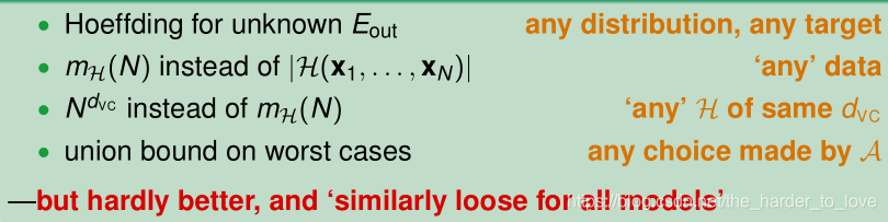
Looseness of VC Bound
N ≈ 10 , 000 d v c in theory , N ≈ 10 d v c in practice N \approx 10,000 d_{\mathrm{vc}} \ \text{in theory},N \approx 10 d_{\mathrm{vc}} \ \text{in practice} N≈10,000dvc in theory,N≈10dvc in practice
我们能基于VC Bound原理提升整个机器学习流程。
Fun Time
Consider the VC Bound below. How can we decrease the probability of getting BAD data?
1 decrease model complexity
d
v
c
d_{\mathrm{vc}}
dvc
2 increase data size
N
N
N a lot
3 increase generalization error tolerance
ϵ
\epsilon
ϵ
4 all of the above
✓
\checkmark
✓
Explanation
降低模型复杂度:减少假设集选择
增大数据量:使训练数据更接近真实数据分布
增大容忍程度:扩大好数据范围
Summary
本篇讲义主要讲了模型复杂度,数据数量级以及VC Bound的宽松程度。
在有限的 d v c d_{\mathrm{vc}} dvc,足够大的 N N N,足够小的 E i n E_{in} Ein,我们真正能学到模型。
讲义总结
Definition of VC Dimension
maximum non-break point
VC Dimension of Perceptrons
d
V
C
(
H
)
=
d
+
1
d_{VC} (H)= d + 1
dVC(H)=d+1
Physical Intuition of VC Dimension
d
V
C
d_{VC}
dVC ≈ #free parameters
Interpreting VC Dimension
loosely: model complexity & sample complexity
参考文献
《Machine Learning Foundations》(机器学习基石)—— Hsuan-Tien Lin (林轩田)


 394
394

 被折叠的 条评论
为什么被折叠?
被折叠的 条评论
为什么被折叠?
 到【灌水乐园】发言


