机器学习基石笔记（八）：噪音和损失

Lecture 8: Noise and Error

Noise and Probabilistic Target

   can replace $f(x)$ by $P(y|x)$

Noise

   noise in y, i.e. good customer, ‘mislabeled’ as bad.
   noise in y: i.e. same customers, different labels.
   noise in x: i.e. inaccurate customer information.

Probabilistic Target

Deterministic Distribution
$$\begin{array}{l}\mathbf{x}\sim P(\mathbf{x})\\ y=f(\mathbf{x})\text{with}P(y|\mathbf{x})=1\\ i.e.P(o|\mathbf{x})=1,P(\times |\mathbf{x})=0\end{array}$$

Probabilistic Distribution
$$\begin{array}{l}\mathbf{x}\sim P(\mathbf{x})\\ y=f(\mathbf{x})\text{with}0\le P(y|\mathbf{x})\le 1\\ i.e.P(o|\mathbf{x})=0.7,P(\times |\mathbf{x})=0.3\end{array}$$
之前阐述的决定分布是概率分布的一种特殊情况（$P(y|\mathbf{x})=1$）。

现在是在概率分布$P(y|\mathbf{x})$中学习，包含$f(\mathbf{x})$和噪音（noise）。

只是在原有的数据分布中，加上条件概率，不影响原来VC Bound的推导及使用。

Fun Time

Let’s revisit PLA/pocket. Which of the following claim is true?
1 In practice, we should try to compute if $D$ is linear separable before deciding to use PLA.
2 If we know that $D$ is not linear separable, then the target function $f$ must not be a linear function.
3 If we know that $D$ is linear separable, then the target function $f$ must be a linear function.
4 None of the above  $✓$


Explanation
1 如果我们可以计算$D$是否线性可分，那么就能直接获取$W^{\ast }$，就无需使用PLA算法。
2 数据集线性不可分，可能存在噪音，真实数据集线性可分
3 数据集线性可分，可能收集的数据少*，存在巧合，并不一定说明目标函数一定是线性函数。?

Error Measure

$$\begin{gathered} E_{\mathrm{i}\mathrm{n}}(g)=\frac{1}{N}\sum _{n=1}^N\mathrm{err}\left(g\left({\mathbf{x}}_n\right),f\left({\mathbf{x}}_n\right)\right) \\ {E}_{\text{out}}(g)=\underset{\mathbf{x}\sim P}{E}\mathrm{err}(g(\mathbf{x}),f(\mathbf{x})) \end{gathered}$$
训练数据是有限的，使用离散分布列计算平均损失。
预测数据是无限的，使用概率分布计算平均损失。
以后会学到测试数据，我们使用测试数据代替预测数据，来判断学习模型的好坏。

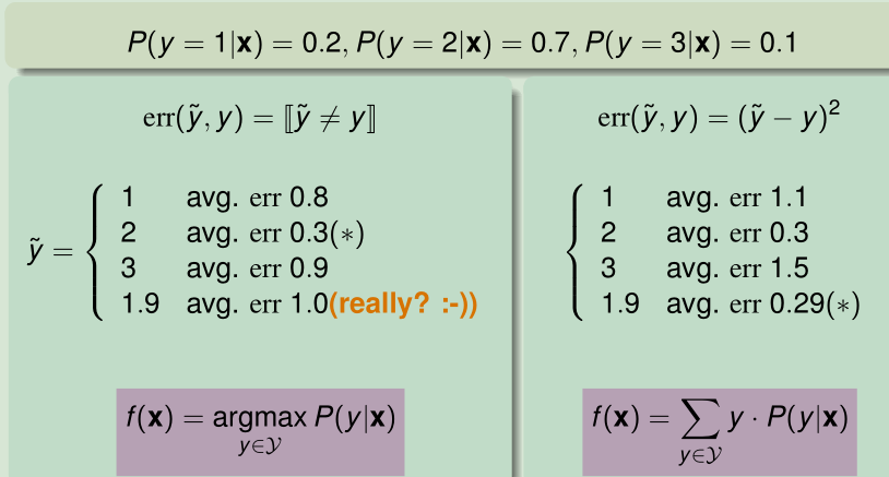
0/1 error

also called classification error.
$$\begin{gathered} \mathrm{err}(\tilde{y},y)=[\tilde{y}̸=y] \\ f(\mathbf{x})=\underset{y\in \mathcal{Y}}{\mathrm{argmax}}P(y|\mathbf{x}) \end{gathered}$$

squared error

$$\begin{gathered} \mathrm{err}(\tilde{y},y)=(\tilde{y}-y{)}^2 \\ f(\mathbf{x})=\sum _{y\in \mathcal{Y}}y\cdot P(y|\mathbf{x}) \end{gathered}$$

   affect ‘ideal’ target

Ideal Mini-Target

$P(y|\mathbf{x})$ and err measure define ideal mini-target $f(\mathbf{x})$.

$A$根据损失衡量方法，选择假设$g$.

Fun Time

Consider the following P(y|x) and err(˜ y,y)|˜ y − y|. Which of the following is the ideal mini-target f(x)?
$$\begin{array}{l}P(y=1|\mathbf{x})=0.10,P(y=2|\mathbf{x})=0.35\\ P(y=3|\mathbf{x})=0.15,P(y=4|\mathbf{x})=0.40\end{array}$$
1 2.5 = average within $Y$ = {1,2,3,4}
2 2.85 = weighted mean from $P(y|\mathbf{x})$
3 3 = weighted median from $P(y|\mathbf{x})$  $✓$
4 4 = $\underset{y\in \mathcal{Y}}{\mathrm{argmax}}P(y|\mathbf{x})$


Explanation
2.5, 2.85, 3, 4的损失目标值分别为1.0, 0.965, 0.95, 1.15.
其实对于绝对值损失衡量方法，最小目标值为中位数计算所得。
至于原因，大家进行一下思维实验。
  现在以中位数计算得到目标值，由于中位数本身占了一定比例，左边+中位数>右边，若往左移，目标值会增大；同理往右移亦然。?

# 计算绝对值损失
def count_absolute_loss(pros, value):
    loss = 0
    for p, v in pros:
        loss += p * math.fabs(v-value)
    return loss

if __name__ == '__main__':
    pros = [(0.1, 1), (0.35, 2), (0.15, 3), (0.4, 4)]
    print(count_absolute_loss(pros, 2.5))  # 1.0
    print(count_absolute_loss(pros, 2.85))  # 0.965
    print(count_absolute_loss(pros, 3))  # 0.95
    print(count_absolute_loss(pros, 4))  # 1.15

Algorithmic Error Measure

Choice of Error Measure

two types of error: false accept and false reject

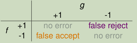
$g$是预测值，$f$是真实值，我们以预测值做决策。

PF：g = +1，f = -1, 错误的接受；

NT：g = -1，f = +1, 错误的拒绝；

0/1 error penalizes both types equally.

Fingerprint Verification for Supermarket

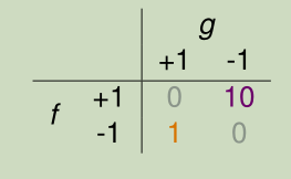
对于超市促销活动来说，错误拒绝比错误接受损失大，增大错误拒绝的损失权值（宁可多发优惠券，不可寒了顾客的心）。

Fingerprint Verification for CIA

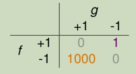
对于CIA审核来说，错误接受比错误拒绝损失大，增大错误接受的损失权值（宁可错抓三千，不可漏放一个）。

$A$从众多损失衡量方法挑选一个损失衡量方法，并确定损失衡量的权重$\widehat{\mathrm{e}\mathrm{r}\mathrm{r}}$，选择假设$g$.

Fun Time

Consider err below for CIA. What is E in (g) when using this err?

1 $\frac{1}{N}\sum _{n=1}^N\left[y_n̸=g\left({\mathbf{x}}_n\right)\right]$
2 $\frac{1}{N}\left(\sum _{y_n=+1}\left[y_n̸=g\left({\mathbf{x}}_n\right)\right]+1000\sum _{y_n=-1}\left[y_n̸=g\left({\mathbf{x}}_n\right)\right]\right)$
3 $\frac{1}{N}\left(\sum _{y_n=+1}\left[y_n̸=g\left({\mathbf{x}}_n\right)\right]-1000\sum _{y_n=-1}\left[y_n̸=g\left({\mathbf{x}}_n\right)\right]\right)$  $✓$
4 $\frac{1}{N}\left(1000\sum _{y_n=+1}\left[y_n̸=g\left({\mathbf{x}}_n\right)\right]+\sum _{y_n=-1}\left[y_n̸=g\left({\mathbf{x}}_n\right)\right]\right)$


Explanation
$g$是预测值，$f$是真实值$y_n$。
注意下权值。?

Weighted Classification

Cost(Error, Loss)
代价又名错误，损失。
$$E_{\mathrm{i}\mathrm{n}}^{\mathrm{W}}(h)=\frac{1}{N}\sum _{n=1}^N\left\{\begin{array}{cc}1& \text{ if }{y}_n=+1\\ 1000& \text{ if }{y}_n=-1\end{array}\right\}\cdot \left[y_n̸=h\left({\mathbf{x}}_n\right)\right]$$

Systematic Route

Connect $E_{in}^w$ and $E_{in}^{0/1}$.

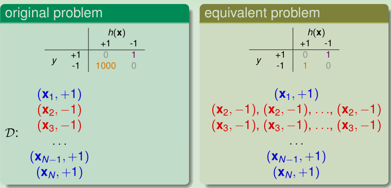
等价于将$y_n=-1$的数据扩大1000倍。
这样在选择到$y_n=-1$的概率增大了。
weighted PLA: 不影响最后的损失偏移（0），若是随机选择数据，会影响PLA的改变过程，导致产生不影响$w^{\ast }$（话说本来随机PLA每次运行就会产生不同$w^{\ast }$）。

weighted pocket ：影响随机过程（若随机选点），影响最终的$w^{\ast }$选择。

Fun Time

Consider the CIA cost matrix. If there are 10 examples with $y_n$ = −1 (intruder) and 999,990 examples with $y_n$ = +1 (you).
What would $E_{\mathrm{i}\mathrm{n}}^{\mathrm{w}}(h)$ be for a constant h(x) that always returns +1?
1 0.001
2 0.01  $✓$
3 0.1
4 1


Explanation
全猜+1,则有10个数据错误，且权重为1000
$\frac{10\ast 1000}{10+999990}=0.01$
权重可以调整不平衡数据带来的影响（若权重全为1，损失目标为0.00001，调大损失权重后，则会增大倾向选择数据多类别的模型的损失，减少模型对数据多类别的倾向）。

Summary

本篇讲义主要讲了噪音，概率目标，损失函数，以及带权重的模型。

在分布函数$P(y|\mathbf{x})$和低损失$E_{in}$下，我们真正能学到模型。

讲义总结

Noise and Probabilistic Target
   can replace $f(x)$ by $P(y|x)$

Error Measure
   affect ‘ideal’ target

Algorithmic Error Measure
   user-dependent $=>$ plausible or friendly

Weighted Classification
   easily done by virtual ‘example copying’

参考文献

《Machine Learning Foundations》(机器学习基石)—— Hsuan-Tien Lin (林轩田)