经典卷积模型(二)LeNet、AlexNetx代码解析

本文链接：https://blog.youkuaiyun.com/sleepinghm/article/details/120075657

本文详细解读了LeNet-5和AlexNet两种经典卷积神经网络模型的结构、代码实现以及在数字识别任务中的应用。LeNet-5以99.2%的准确率在MNIST上脱颖而出，而AlexNet的8层结构和深度学习特征提取过程也被逐一剖析。

摘要生成于 C知道，由 DeepSeek-R1 满血版支持，前往体验 >

LeNet-5

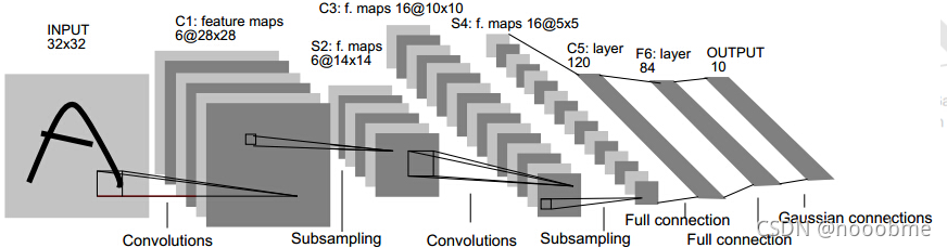
LeNet-5，它是第一个成功应用于数字识别的卷积神经网络。在MNIST数据集上，可以达到99.2%的准确率。
LeNet-5模型总共有7层，包括两个卷积层，两个池化层，两个全连接层和一个输出层。
在这里插入图片描述
代码实现：

class LeNet(nn.Module):
    def __init__(self):
        super(LeNet,self).__init__()
        self.conv1=nn.Conv2d(3,6,5)
        self.conv2=nn.Conv2d(6,16,5)
        self.fc1=nn.Linear(16*5*5,120)
        self.fc2=nn.Linear(120,84)
        self.fc3=nn.Linear(84,10)
    def forward(self,x):
        out=F.relu(self.conv1(x))
        out=F.max_pool2d(out,2)
        out=F.relu(self.conv2(out))
        out=F.max_pool2d(out,2)
        out=out.view(out.size(0),-1)
        out=F.relu(self.fc1(out))
        our=F.relu(self.fc2(out))
        out=self.fc3(out)
        return out

假设图片长宽32*32且通道数为3，忽略batchsize，维度为(32,32,3)。看forward部分：

第一步out=F.relu(self.conv1(x))：其中conv1=nn.Conv2d(3,6,5)，即将3通道数扩增到6，卷积核大小为5*5，可以算出来特征图的输出大小为(32-5+2*0)/1+1=28，即(32,32,3)->(28,28,6)。共有28*28*6个神经元，5*5*6+6个参数量。
第二步F.max_pool2d(out,2)：最大池化层，二倍下采样，即(28,28,6)->(14,14,6)。
第三步out=F.relu(self.conv2(out))：其中conv2=nn.Conv2d(6,16,5)，通道数从6->16，卷积核大小5*5，则输出大小(14-5+2*0)/1+1=10，即(14,14,6)->(10,10,16)。
第四步F.max_pool2d(out,2)：同第二步，即(10,10,16)->(5,5,16)。
第五步out.view(out.size(0),-1)：打平维度，将(5,5,16)->(5*5*16=240)。
第六步F.relu(self.fc1(out))：fc1=nn.Linear(16*5*5,120)，全连接层，将(240)->(120)。
第七步F.relu(self.fc2(out))：self.fc2=nn.Linear(120,84)，全连接层，将(120)->(84)。
第八步out=self.fc3(out)：self.fc3=nn.Linear(84,10)，全连接层也是最终输出层，将(84)->(10)，最终输出10维度，代表手写数字识别0~9。

AlexNet

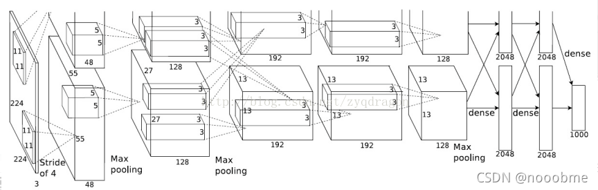
AlexNet共8层，前5层为卷积层，后3层为全连接层。
在这里插入图片描述
官方代码，移除了LRN。

class AlexNet(nn.Module):
    def __init__(self, num_classes: int = 1000) -> None:
        super(AlexNet, self).__init__()
        self.features = nn.Sequential(
        	#1
            nn.Conv2d(3, 64, kernel_size=11, stride=4, padding=2),
            nn.ReLU(inplace=True),
            nn.MaxPool2d(kernel_size=3, stride=2),
            #2
            nn.Conv2d(64, 192, kernel_size=5, padding=2),
            nn.ReLU(inplace=True),
            nn.MaxPool2d(kernel_size=3, stride=2),
            #3
            nn.Conv2d(192, 384, kernel_size=3, padding=1),
            nn.ReLU(inplace=True),
            #4
            nn.Conv2d(384, 256, kernel_size=3, padding=1),
            nn.ReLU(inplace=True),
            #5
            nn.Conv2d(256, 256, kernel_size=3, padding=1),
            nn.ReLU(inplace=True),
            nn.MaxPool2d(kernel_size=3, stride=2),
        )
        #6
        self.avgpool = nn.AdaptiveAvgPool2d((6, 6))
        self.classifier = nn.Sequential(
        	#7
            nn.Dropout(),
            nn.Linear(256 * 6 * 6, 4096),
            nn.ReLU(inplace=True),
            #8
            nn.Dropout(),
            nn.Linear(4096, 4096),
            nn.ReLU(inplace=True),
            #9
            nn.Linear(4096, num_classes),
        )

    def forward(self, x: torch.Tensor) -> torch.Tensor:
        x = self.features(x)
        x = self.avgpool(x)
        x = torch.flatten(x, 1)
        x = self.classifier(x)
        return x

图片大小224*224，通道为3，所以输入维度为（224，224，3）。
在forward部分分为x=self.features()也就是卷积部分，得到卷积后的特征；x=x.view(x.size(0),256*6*6)，将特征打平送入分类层；x=self.classifier(x)，分类输出。以下忽略激活函数和dropout部分。

使用了卷积核大小11*11，步长为4，填充为2的卷积核，卷积核数量96个，将3通道扩展到96，输出特征大小为(224-11+2*2)/4+1=55。随后使用2倍下采样的最大池化层，即(224,224,3)->(55,55,96)->(27,27,96)。
```
   nn.Conv2d(3, 64, kernel_size=11, stride=4, padding=2),
   nn.ReLU(inplace=True),
   nn.MaxPool2d(kernel_size=3, stride=2),
```
使用了卷积核大小5*5，填充为2的卷积核，卷积核数量192个，将96通道扩展到192，输出特征大小为(27-5+2*2)/1+1=27，大小保持不变，然后使用2倍下采样的最大池化层，即(27,27,96)->(27,27,192)->(13,13,192)。
```
nn.Conv2d(64, 192, kernel_size=5, padding=2),
nn.ReLU(inplace=True),
nn.MaxPool2d(kernel_size=3, stride=2),
```
使用了卷积核大小3*3，填充为1的卷积核，卷积核数量384个，将192通道扩展到384，输出特征大小为(13-3+2*1)/1+1=13，大小保持不变，即(13,13,192)->(13,13,384)。
```
nn.Conv2d(192, 384, kernel_size=3, padding=1),
nn.ReLU(inplace=True),
```
使用了卷积核大小3*3，填充为1的卷积核，卷积核数量256个，将384通道缩减到256，通道数保持不变，输出特征大小为(13-3+2*1)/1+1=13，大小也保持不变，即((13,13,384)->(13,13,256)。
```
nn.Conv2d(384, 256, kernel_size=3, padding=1),
nn.ReLU(inplace=True),
```
使用了卷积核大小3*3，填充为1的卷积核，卷积核数量256个，通道保持不变，输出特征大小为(13-3+2*1)/1+1=13，大小保持不变，然后使用2倍下采样的最大池化层，即(13,13,256)->(13,13,256)->(6,6,256)。
```
nn.Conv2d(256, 256, kernel_size=3, padding=1),
nn.ReLU(inplace=True),
nn.MaxPool2d(kernel_size=3, stride=2),
```
经过自适应平均池化层，将大小缩减为(6, 6)，则(13,13,256)->(6,6,256)。
```
self.avgpool = nn.AdaptiveAvgPool2d((6, 6))
```
现在进入分类部分。在分类之前x = torch.flatten(x, 1)，因此此时特征为(6,6,256)->(6*6*256)。然后使用全连接层nn.Linear(256*6*6,4096)，将特征(256*6*6)->(4096)。
```
nn.Dropout(),
nn.Linear(256*6*6,4096),
nn.ReLU(inplace=True),
```
使用全连接层nn.Linear(4096,4096)，将特征(4096)->(4096)，保持不变，增加非线性。
```
  nn.Dropout(),
  nn.Linear(4096,4096),
  nn.ReLU(inplace=True),
```
最终输出层，使用nn.Linear(4096,num_classes)的全连接层，将4096维度分类成num_classes的个数。

补充

LRN（local response normalization）局部响应标准化
LRN函数类似DROPOUT和数据增强作为relu激励之后防止数据过拟合而提出的一种处理方法。这个函数很少使用，基本上被类似DROPOUT这样的方法取代，见最早的出处AlexNet论文对它的定义。
nn.ReLU(inplace=True)中inplace的作用
inplace-选择是否进行覆盖运算，nn.ReLU(inplace=True) 的意思就是对从上层网络Conv2d中传递下来的tensor直接进行修改，这样能够节省运算内存，不用多存储其他变量。否则就需要花费内存去多存储一个变量
nn.Dropout()
nn.Dropout( p ), 默认p=0.5，Dropout的目的是防止过拟合，dropout层不会影响模型的shape。