YOLOv13超图自适应增强

原创已于 2025-08-14 21:27:49 修改 · 2k 阅读

53 ·

CC 4.0 BY-SA版权

文章标签：

#YOLO

于 2025-08-14 21:05:00 首次发布

CV 专栏收录该内容

3 篇文章

订阅专栏

YOLOV13超图卷积

前言

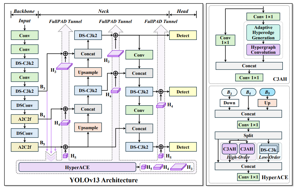
YOLO系列已经来到了V13版本，其提出的基于超图的自适应相关性增强（HyperACE）机制能够自适应地利用潜在的高阶关联，实现了高效的全局跨位置和跨尺度特征融合与增强，克服了以往方法仅限于基于超图计算的成对相关性建模的局限性。本文将图解超图卷积的过程，并结合YOLOv13的代码提供一个即插即用的HGNN（超图神经网络模块），方便大家进行二次创新。
在这里插入图片描述

图神经网络

图神经网络（Graph Neural Networks, GNN）通过学习节点之间的关系和图的拓扑结构来进行节点分类、图分类和链接预测等任务。图神经网络的核心思想是通过消息传递和节点更新的方式，使每个节点能够从其邻居节点中获取信息并更新自身的表征向量。
在这里插入图片描述

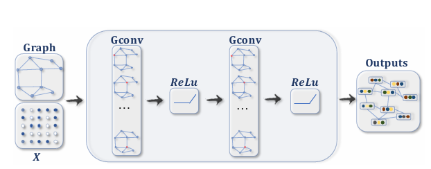
想要详细了解图卷积的同路人可以阅读一下图神经网络的综述文章A Comprehensive Survey on Graph Neural
Networks

超图神经网络

有了图神经网络的了解，我们再来了解一下超图神经网络。不可否认在深度学习中，对象之间的关系是高阶的，因此超图神经网络应运而生，可以更加灵活的表示各节点特征间的高阶关系，即使用动态生成超边的方法，这就是超图神经网络。
在这里插入图片描述
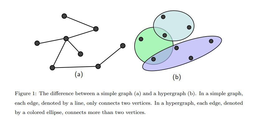
超图神经网络充分利用特征间的高阶关系和局部聚类结构来实现顶点之间的有效信息传播。显著区别于图神经网络，超图神经网络没有并没有将特征汇集于一个特征顶点，而是通过超图关系聚合特征。假设超图表示为 $G = (V, E)$ ，具有N个特征向量(顶点)，M个超边。V表示所有特征向量的集合 $V=\{v1,v2,...,vN\}$ ，E表示超边集合 $\subseteq V \times V$ ，W为记录各条超边的权重的对角矩阵 $\in M \times M$ 。
如果节点vi包含在超边 $\in E$ 中，则 $H i e = 1$ ，否则为0。此时，节点的度可以定义为：
${D_{ii}} = \sum\limits_{e = 1}^M {{W_{ee}}} {H_{ie}}$
超边的度可以定义为：
${B_{ee}} = \sum\limits_{i = 1}^N {{H_{ie}}}$
节点的度矩阵和超边的度矩阵都是对角矩阵。
则超图卷积可以定义为：
${X^{(l + 1)}} = \sigma ({D^{ - 1/2}}HW{B^{ - 1}}HT{D^{ - 1/2}}{X^{(l)}}P)$
可以参考下面这篇文章进一步理解：
Hypergraph Convlution and Hypergraph Attention

YOLOv13超图卷积图解

在这里插入图片描述
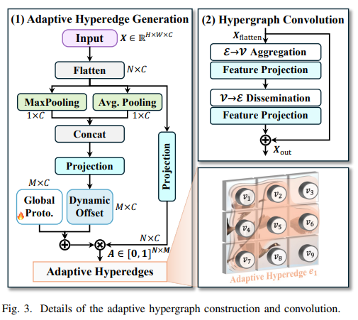
基于超图的自适应相关增强 (HyperACE) 机制是YOLOv13的核心创新点，在自适应超图中，每个超边收集来自所有顶点的特征，每一个顶点在这个超图中的参与度表示顶点的在这个图关系中的重要性。主要的部分由以上两部分构成，即超边生成和超图卷积两个部分。

超边生成

自适应超边缘生成阶段的重点是根据输入的视觉特征动态建模相关性，以生成超边缘并估计每个顶点对每个超边缘的参与程度。在Fig3的左图中对超边生成的过程描述已经很全面了，首先在通道维度分别进行最大和平均池化，接着将两个特征进行拼接，然后通过线性层生成 $\times N$ 维的向量进行高阶关系的代理向量，并通过Global Proto增加固有的可学习偏执，此时代理向量的维度为 $（ BMC ）$ ，其中B为批大小、M为超边个数、C为输入图像的通道数，最后通过矩阵乘法与输入打平后的特征图进行相关性计算，类似于多头注意力的计算，不过查询的维度变小了，然后在每一个头里面做了平均来计算每一个超边中每一个特征层的权重。
生成超边的代码如下：

B, N, D = x.shape
        if self.context == "mean":
            context_cat = x.mean(dim=1)
        elif self.context == "max":
            context_cat, _ = x.max(dim=1)
        else:
            avg_context = x.mean(dim=1)
            max_context, _ = x.max(dim=1)
            context_cat = torch.cat([avg_context, max_context], dim=-1)
        #左侧的Projection 定义的是Linear层
        prototype_offsets = self.context_net(context_cat).view(B, self.num_hyperedges, D)
        #增加固有偏置
        prototypes = self.prototype_base.unsqueeze(0) + prototype_offsets
		#右侧的Projection定义的是Linear层
        X_proj = self.pre_head_proj(x)
        #维度变换
        X_heads = X_proj.view(B, N, self.num_heads, self.head_dim).transpose(1, 2)
        proto_heads = prototypes.view(B, self.num_hyperedges, self.num_heads, self.head_dim).permute(0, 2, 1, 3)

        X_heads_flat = X_heads.reshape(B * self.num_heads, N, self.head_dim)
        proto_heads_flat = proto_heads.reshape(B * self.num_heads, self.num_hyperedges, self.head_dim).transpose(1, 2)
		#x_head     -> B*num_head  W*H head_dim
		#prototypes -> B*num_head num_edge head_dim
        logits = torch.bmm(X_heads_flat, proto_heads_flat) / self.scaling
        #在每一个相关性计算的头上取了平均值
        logits = logits.view(B, self.num_heads, N, self.num_hyperedges).mean(dim=1)
		#生成的超边为 B W*H num_edge
		#输出通过softmax范围为0-1
        return F.softmax(logits, dim=1)

在这里插入图片描述
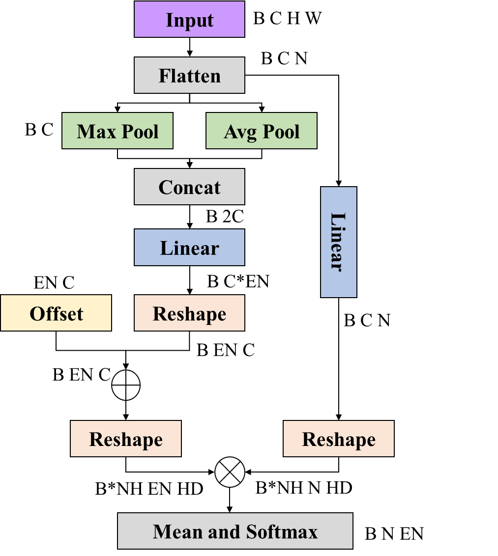
其中EN代表超边的个数，NH代表相关性计算头的个数，HD代表计算的维度。

超图计算

超图计算利用依据相关性计算得出的超图关系进行聚合各特征层的特征，汇聚后使用线性层和GeLU激活函数进行特征的加强，接着使用加强后的特征通过超边映射回各特征层形成新的特征加强后的特征层，最后再通过线性层和GeLU激活函数进行特征的再次增强。
在这里插入图片描述
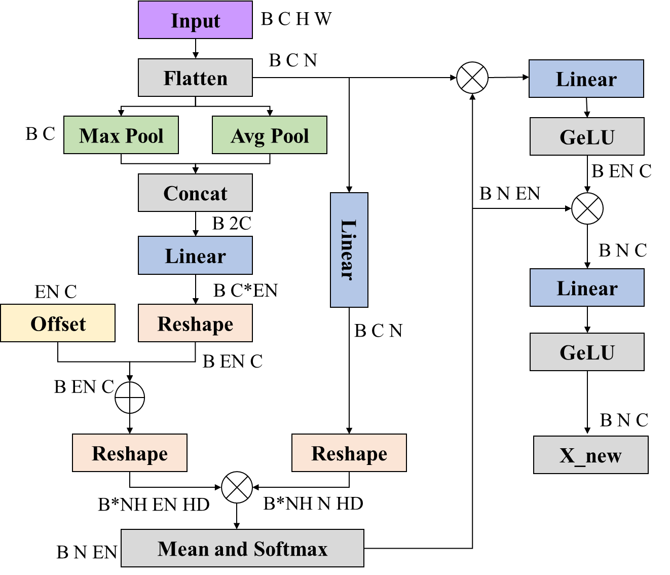
如果需要残差连接就再加上Flatten后的输入。
到这里YOLOv13的超图卷积的超图计算就讲完了，个人感觉可以即插即用在任何卷积、Ateention、一维二维甚至三维的的深度学习任务中，我将其封装成了一个超图神经网络模块方便大家使用。

超图神经网络

class HGNN(nn.Module):
    def __init__(self,node_dim, num_hyperedges, num_heads=4, context="both"):
        super(HGNN, self).__init__()
        self.num_heads = num_heads
        self.num_hyperedges = num_hyperedges
        self.head_dim = node_dim // num_heads
        self.context = context

        if context in ("mean", "max"):
            self.context_net = nn.Linear(node_dim, num_hyperedges * node_dim)
        elif context == "both":
            self.context_net = nn.Linear(2 * node_dim, num_hyperedges * node_dim)
        else:
            raise ValueError(
                f"Unsupported context '{context}'. "
                "Expected one of: 'mean', 'max', 'both'."
            )
        self.prototype_base = nn.Parameter(torch.Tensor(num_hyperedges, node_dim))
        nn.init.xavier_uniform_(self.prototype_base)
        self.pre_head_proj = nn.Linear(node_dim, node_dim)
        self.scaling = self.head_dim ** -0.5

        self.edge_proj = nn.Sequential(
            nn.Linear(node_dim, node_dim),
            nn.GELU()
        )
        self.node_proj = nn.Sequential(
            nn.Linear(node_dim, node_dim),
            nn.GELU()
        )

    def generate_hyperedges(self,x):
        B, N, D = x.shape
        if self.context == "mean":
            context_cat = x.mean(dim=1)
        elif self.context == "max":
            context_cat, _ = x.max(dim=1)
        else:
            avg_context = x.mean(dim=1)
            max_context, _ = x.max(dim=1)
            context_cat = torch.cat([avg_context, max_context], dim=-1)
        prototype_offsets = self.context_net(context_cat).view(B, self.num_hyperedges, D)
        prototypes = self.prototype_base.unsqueeze(0) + prototype_offsets

        X_proj = self.pre_head_proj(x)
        X_heads = X_proj.view(B, N, self.num_heads, self.head_dim).transpose(1, 2)
        proto_heads = prototypes.view(B, self.num_hyperedges, self.num_heads, self.head_dim).permute(0, 2, 1, 3)

        X_heads_flat = X_heads.reshape(B * self.num_heads, N, self.head_dim)
        proto_heads_flat = proto_heads.reshape(B * self.num_heads, self.num_hyperedges, self.head_dim).transpose(1, 2)

        logits = torch.bmm(X_heads_flat, proto_heads_flat) / self.scaling
        logits = logits.view(B, self.num_heads, N, self.num_hyperedges).mean(dim=1)

        return F.softmax(logits, dim=1)

    def forward(self, X):
        # B N D
        A = self.generate_hyperedges(X)
        He = torch.bmm(A.transpose(1, 2), X)
        He = self.edge_proj(He)
        X_new = torch.bmm(A, He)
        X_new = self.node_proj(X_new)
        return X_new