


前言
本篇文章是深度学习第四周的实验内容,主要使用pytorch来实现线性分类模型,二分类,多分类,并且利用softmax回归完成鸢尾花数据集分类任务,我们一起来学习吧(ง •_•)ง
pytorch实现
第3章 线性分类
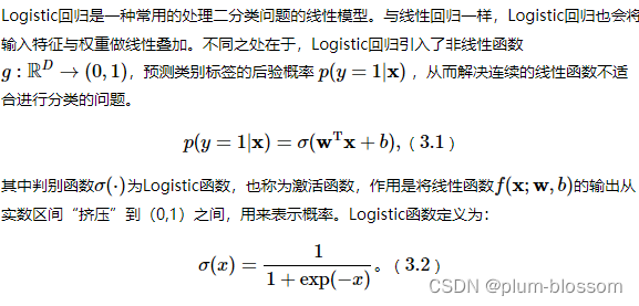
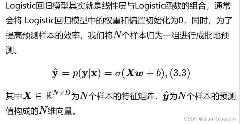
3.1 基于Logistic回归的二分类任务
3.1.1 数据集构建
构建一个简单的分类任务,并构建训练集、验证集和测试集。
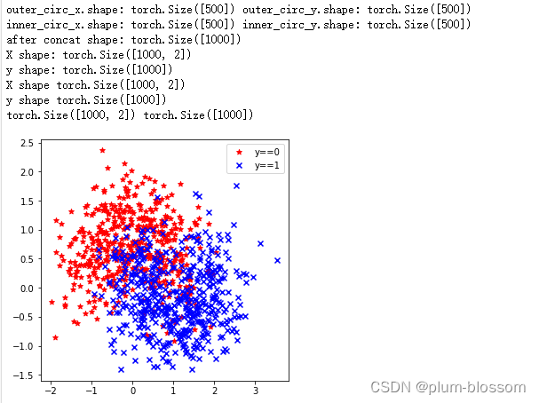
本任务的数据来自带噪音的两个弯月形状函数,每个弯月对一个类别。我们采集1000条样本,每个样本包含2个特征。
随机采集1000个样本,并进行可视化。
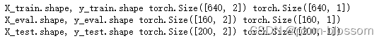
将1000条样本数据拆分成训练集、验证集和测试集,其中训练集640条、验证集160条、测试集200条。
先导入后续需要使用的函数:
import numpy as np
import pandas as pd
%matplotlib inline
import matplotlib.pyplot as plt
import torch
import math
生成弯月形状的函数代码如下:
def make_moons(n_samples=1000, shuffle=True, noise=None):
    """
    生成带噪音的弯月形状数据
    输入:
        - n_samples:数据量大小,数据类型为int
        - shuffle:是否打乱数据,数据类型为bool
        - noise:以多大的程度增加噪声,数据类型为None或float,noise为None时表示不增加噪声
    输出:
        - X:特征数据,shape=[n_samples,2]
        - y:标签数据, shape=[n_samples]
    """
    n_samples_out = n_samples // 2
    n_samples_in = n_samples - n_samples_out


    outer_circ_x = torch.cos(torch.linspace(0, math.pi, n_samples_out))
    outer_circ_y = torch.sin(torch.linspace(0, math.pi, n_samples_out))

    inner_circ_x = 1 - torch.cos(torch.linspace(0, math.pi, n_samples_in))
    inner_circ_y = 0.5 - torch.sin(torch.linspace(0, math.pi, n_samples_in))

    print('outer_circ_x.shape:', outer_circ_x.shape, 'outer_circ_y.shape:', outer_circ_y.shape)
    print('inner_circ_x.shape:', inner_circ_x.shape, 'inner_circ_y.shape:', inner_circ_y.shape)

    # 使用'torch.concat'将两类数据的特征1和特征2分别延维度0拼接在一起,得到全部特征1和特征2
    # 使用'torch.stack'将两类特征延维度1堆叠在一起
    X = torch.stack(
        [torch.concat([outer_circ_x, inner_circ_x]),
        torch.concat([outer_circ_y, inner_circ_y])],
        axis=1
    )

    print('after concat shape:', torch.concat([outer_circ_x, inner_circ_x]).shape)
    print('X shape:', X.shape)

    # 使用'torch. zeros'将第一类数据的标签全部设置为0
    # 使用'torch. ones'将第一类数据的标签全部设置为1
    y = torch.concat(
        [torch.zeros(n_samples_out), torch.ones(n_samples_in)]
    )

    print('y shape:', y.shape)

    # 如果shuffle为True,将所有数据打乱
    if shuffle:
        # 使用'torch.randperm'生成一个数值在0到X.shape[0],随机排列的一维Tensor做索引值,用于打乱数据
        idx = torch.randperm(X.shape[0])
        X = X[idx]
        y = y[idx]
        print('X shape', X.shape)
        print('y shape', y.shape)

    # 如果noise不为None,则给特征值加入噪声
    if noise is not None:
        # 使用'torch.normal'生成符合正态分布的随机Tensor作为噪声,并加到原始特征上
        X += torch.normal(0, noise, size=X.shape)

    return X, y
随机采取1000个样本,,并进行可视化:
# 采样1000个样本
n_samples = 1000
X, y = make_moons(n_samples=n_samples, shuffle=True, noise=0.5)
# 可视化生产的数据集,不同颜色代表不同类别

print(X.shape, y.shape)

plt.figure(figsize=(5,5))
plt.scatter(x=X[:, 0][y==0], y=X[:, 1][y==0], marker='*', c='red', label='y==0')
plt.scatter(x=X[:, 0][y==1], y=X[:, 1][y==1], marker='x', c='blue', label='y==1')
plt.legend()
plt.show()
运行结果:
划分数据集:
由于在生成数据的时候已经进行过shuffle,在划分数据的时候不用再次打乱数据。
代码如下:
train_num = 640
eval_num = 160
test_num = 200

X_train, y_train = X[: train_num], y[: train_num]
X_eval, y_eval = X[train_num: train_num+eval_num], y[train_num: train_num+eval_num]
X_test, y_test = X[train_num+eval_num: ], y[train_num+eval_num: ]

y_train = y_train.reshape([-1, 1])
y_eval = y_eval.reshape([-1,1])
y_test = y_test.reshape([-1,1])

print('X_train.shape, y_train.shape', X_train.shape, y_train.shape)
print('X_eval.shape, y_eval.shape', X_eval.shape, y_eval.shape)
print('X_test.shape, y_test.shape', X_test.shape, y_test.shape)
运行结果:
3.1.2 模型构建
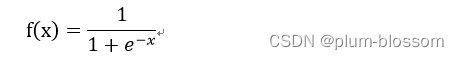
# 定义Logistic函数
def logistic(x):
return 1 / (1 + torch.exp(-x))
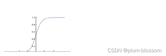
# 绘制logistic函数图像
# 在[-10,10]的范围内生成一系列的输入值,用于绘制函数曲线
x = torch.linspace(-10, 10, 10000)
plt.figure()
plt.plot(x, logistic(x), color="#e4007f", label="Logistic Function")
# 设置坐标轴
ax = plt.gca()
# 取消右侧和上侧坐标轴
ax.spines['top'].set_color('none')
ax.spines['right'].set_color('none')
# 设置默认的x轴和y轴方向
ax.xaxis.set_ticks_position('bottom')
ax.yaxis.set_ticks_position('left')
# 设置坐标原点为(0,0)
ax.spines['left'].set_position(('data',0))
ax.spines['bottom'].set_position(('data',0))
# 添加图例
plt.legend()
plt.savefig('linear-logistic.pdf')
plt.show()
运行结果:
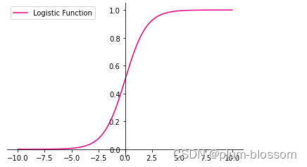
从输出结果看,当输入在0附近时,Logistic函数近似为线性函数;而当输入值非常大或非常小时,函数会对输入进行抑制。输入越小,则越接近0;输入越大,则越接近1。正因为Logistic函数具有这样的性质,使得其输出可以直接看作为概率分布。
Logistic回归算子
class model_LR(Op):
    def __init__(self, input_dim):
        super(model_LR, self).__init__()
        self.params = {

   }
        # 将线性层的权重参数全部初始化为0
        self.params['w'] = torch.zeros([input_dim, 1])
        # self.params['w'] = paddle.normal(mean=0, std=0.01, shape=[input_dim, 1])
        # 将线性层的偏置参数初始化为0
        self.params['b'] = torch.zeros([1])

    def __call__(self, inputs):
        return self.forward(inputs)

    def forward(self, inputs):
        """
        输入:
            - inputs: shape=[N,D], N是样本数量,D为特征维度
        输出:
            - outputs:预测标签为1的概率,shape=[N,1]
        """
        # 线性计算
        score = torch.matmul(inputs, self.params['w']) + self.params['b']
        # Logistic 函数
        outputs = logistic(score)
        return outputs
测试一下
随机生成3条长度为4的数据输入Logistic回归模型,观察输出结果。
# 固定随机种子,保持每次运行结果一致
torch.seed()
# 随机生成3条长度为4的数据
inputs = torch.randn([3,4])
print('Input is:', inputs)
# 实例化模型
model = model_LR(4)
outputs = model(inputs)
print('Output is:', outputs)
运行结果:
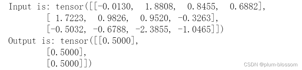
从输出结果看,模型最终的输出g(⋅)恒为0.5。这是由于采用全0初始化后,不论输入值的大小为多少,Logistic函数的输入值恒为0,因此输出恒为0.5。
问题1:Logistic回归在不同的书籍中,有许多其他的称呼,具体有哪些?你认为哪个称呼最好?
在李航的《统计学习方法(第二版)》中被称为逻辑斯蒂分布。
还有对数几率回归。
对数几率回归更好。对数几率函数,简称对率函数。从对数几率回归这个名字就能得知它采用了对数几率函数,比较清楚。
问题2:什么是激活函数?为什么要用激活函数?常见激活函数有哪些?
激活函数的定义:
激活函数,就是在人工神经网络的神经元上运行的函数,负责将神经元的输入映射到输出端。
激活函数对于人工神经网络模型去学习、理解非常复杂和非线性的函数来说具有十分重要的作用。它们将非线性特性引入到我们的网络中。
为什么要使用激活函数:
把非线性特性引入到神经网络中。
如果不使用激活函数,每一层输出都是上层输入的线性函数,无论神经网络有多少层,输出都是输入的线性组合,这种情况就是最原始的感知机。如果使用的话,激活函数给神经元引入了非线性因素,使得神经网络可以任意逼近任何非线性函数,这样神经网络就可以应用到众多的非线性模型中。
常见的激活函数:
Sigmoid函数:
图像如下:
它能够把输入的连续实值变换为0和1之间的输出。如果是非常大的负数,那么输出就是0;如果是非常大的正数,输出就是1。可以用来做二分类。
tanh函数
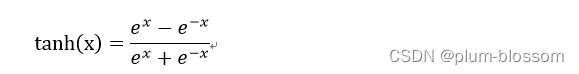
图像如下:
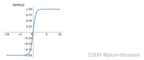
取值范围为[-1,1],
tanh在特征相差明显时效果会很好,在循环过程中会不断扩大特征效果,
tahn是0均值的,在实际应用中tanh比sigmoid更好。
relu函数
relu函数是一个取最大值函数,是目前最常用的激活函数

图像如下
 最低0.47元/天 解锁文章


 2350
2350

 被折叠的 条评论
为什么被折叠?
被折叠的 条评论
为什么被折叠?
 到【灌水乐园】发言


