ADS-Lecture 12 Introduction to Asymptotic Analysis

Lecture 12 Introduction to Asymptotic Analysis

Writing Efficient Programs

An engineer will do for a dime what any fool will do for a dollar.

Efficiency comes in two flavors:

• Programming cost (course to date. Will also revisit later).

  • How long does it take to develop your programs?
  • How easy is it to read, modify, and maintain your code?
    • More important than you might think!
    • Majority of cost is in maintenance, not development!

• Execution cost (from today until end of course).

  • How much time does your program take to execute?
  • How much memory does your program require?

Example of Algorithm Cost

Objective: Determine if a sorted array contains any duplicates.

• Given sorted array A, are there indices i and j where A[i] = A[j]?

Silly algorithm: Consider every possible pair, returning true if any match.

• Are (-3, -1) the same? Are (-3, 2) the same? …

Better algorithm?

• For each number A[i], look at A[i+1], and return true the first time you see a match. If you run out of items, return false.

Today’s goal: Introduce formal technique for comparing algorithmic efficiency.

Intuitive Runtime Characterizations

How Do I Runtime Characterization?

Our goal is to somehow characterize the runtimes of the functions below.

• Characterization should be simple and mathematically rigorous.

• Characterization should demonstrate superiority of dup2 over dup1.

public static boolean dup1(int[] A) {  
    for (int i = 0; i < A.length; i += 1) {
        for (int j = i + 1; j < A.length; j += 1) {
            if (A[i] == A[j]) {
                return true;
            }
        }
    }
    return false;
}
//dup1

public static boolean dup2(int[] A) {
    for (int i = 0; i < A.length - 1; i += 1) {
        if (A[i] == A[i + 1]) { 
            return true; 
        }
    }
    return false;
}
//dup2

Techniques for Measuring Computational Cost

Technique 1: Measure execution time in seconds using a client program.

• Tools:
  • Physical stopwatch.
  • Unix has a built in time command that measures execution time.
  • Princeton Standard library has a Stopwatch class.

Time Measurements for dup1 and dup2

Time to complete(in seconds):

N	dup1	dup2
10000	0.08	0.08
50000	0.32	0.08
100000	1.00	0.08
200000	8.26	0.1
400000	15.4	0.1

[外链图片转存失败,源站可能有防盗链机制,建议将图片保存下来直接上传(img-M0RLsQ7B-1612400444101)(C:\Users\23051\AppData\Roaming\Typora\typora-user-images\image-20210203160501499.png)]

Technique 1: Measure execution time in seconds using a client program.

• Good: Easy to measure, meaning is obvious.

• Bad: May require large amounts of computation time. Result varies with machine, compiler, input data, etc.

Technique 2A: Count possible operations for an array of size N = 10,000.

• Good: Machine independent. Input dependence captured in model.

• Bad: Tedious to compute. Array size was arbitrary. Doesn’t tell you actual time.

Technique 2B: Count possible operations in terms of input array size N.

• Good: Machine independent. Input dependence captured in model. Tells you how algorithm scales.

• Bad: Even more tedious to compute. Doesn’t tell you actual time.

Comparing Algorithms

Which algorithm is better? dup2. Why?

• Fewer operations to do the same work [e.g. 50,015,001 vs. 10000 operations].

• Better answer: Algorithm scales better in the worst case. (N2+3N+2)/2 vs. N.

• Even better answer: Parabolas (N2) grow faster than lines (N).

dup1:

operation	symbolic count	count, N = 10000
i = 0	1	1
j = i + 1	1 to N	1 to 10000
less than(<)	2 to (N^2 + 3N + 2) / 2	2 to 50,015,001
increment (+=1)	0 to (N^2 + N) / 2	0 to 50,005,000
equals(==)	1 to (N^2 - N) / 2	1 to 49,995,000
array accesses	2 to N^2 - N	2 to 99,990,000

dup2:

operation	symbolic count	count, N = 10000
i = 0	1	1
less than(<)	0 to N	2 to 10000
increment (+=1)	0 to N - 1	0 to 9999
equals(==)	1 to N - 1	1 to 9999
array accesses	2 to 2N - 2	2 to 19998

Asymptotic Behavior

In most cases, we care only about asymptotic behavior, i.e. what happens for very large N.

• Simulation of billions of interacting particles.

• Social network with billions of users.

• Logging of billions of transactions.

• Encoding of billions of bytes of video data.

Algorithms which scale well (e.g. look like lines) have better asymptotic runtime behavior than algorithms that scale relatively poorly (e.g. look like parabolas).

Parabolas vs. Lines

Suppose we have two algorithms that zerpify a collection of N items.

• zerp1 takes 2N^2 operations.

• zerp2 takes 500N operations.

For small N, zerp1 might be faster, but as dataset size grows, the parabolic algorithm is going to fall farther and farther behind (in time it takes to complete).

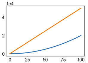
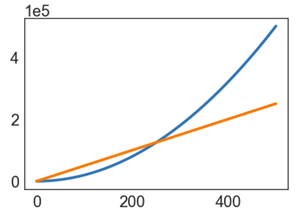
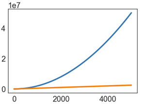
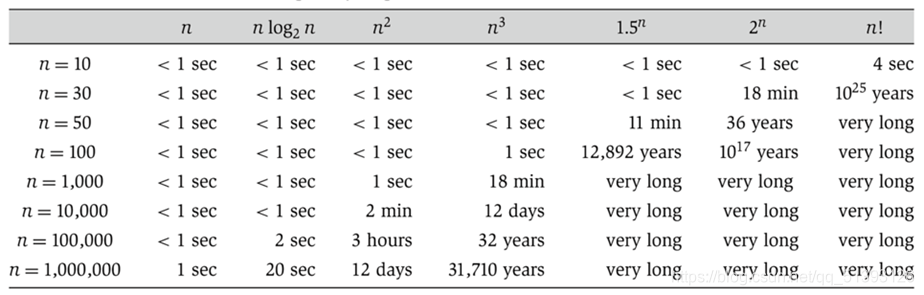
Scaling Across Many Domains

We’ll informally refer to the “shape” of a runtime function as its order of growth (will formalize soon).

• Effect is dramatic! Often determines whether a problem can be solved at all.

Worst Case Order of Growth

Intuitive Simplification 1: Consider Only the Worst Case

Justification: When comparing algorithms, we often care only about the worst case [but we will see exceptions in this course].

We’re effectively focusing on the case where there are no duplicates, because this is where there is a performance difference.

Intuitive Order of Growth Identification

operation	count
less than (<)	100N^2 + 3N
greater than(>)	2N^3 + 1
and(&&)	5,000

Argument:

• Suppose < takes α nanoseconds, > takes β nanoseconds, and && takes γ nanoseconds.

• Total time is α(100N2 + 3N) + β(2N3 + 1) + 5000γ nanoseconds.

• For very large N, the 2βN3 term is much larger than the others.

  Extremely important point. Make sure you understand it!

Intuitive Simplification 2: Restrict Attention to One Operation

Simplification 2: Pick some representative operation to act as a proxy for the overall runtime.

• Good choice: increment.

  • There are other good choices.

• Bad choice: assignment of j = i + 1.

We call our choice the “cost model”.

operation	worst case count
increment(+=1)	(N^2 + N) / 2

Intuitive Simplification 3: Eliminate low order terms.

Simplification 3: Ignore lower order terms.

operation	worst case
increment(+=1)	n^2 / 2

Intuitive Simplification 4: Eliminate multiplicative constants.

Simplification 4: Ignore multiplicative constants.

• Why? It has no real meaning. We already threw away information when we chose a single proxy operation.

operation	worst case
increment(+=1)	N^2

Simplification Summary

Simplifications:

1. Only consider the worst case.

2. Pick a representative operation (a.k.a. the cost model).

3. Ignore lower order terms.

4. Ignore multiplicative constants.

Last three simplifications are OK because we only care about the “order of growth” of the runtime.

Worst case order of growth of runtime: N^2

Simplified Analysis

Simplified Analysis Process

Rather than building the entire table, we can instead:

• Choose a representative operation to count (a.k.a. cost model).

• Figure out the order of growth for the count of the representative operation by either:

  • Making an exact count, then discarding the unnecessary pieces.
  • Using intuition and inspection to determine order of growth (only possible with lots of practice).

Let’s redo our analysis of dup1 with this new process.

• This time, we’ll show all our work.

Analysis of Nested For Loops (Based on Exact Count)

Find the order of growth of the worst case runtime of dup1.

int N = A.length;
for (int i = 0; i < N; i += 1)
    for (int j = i + 1; j < N; j += 1)
        if (A[i] == A[j])
            return true;
return false;

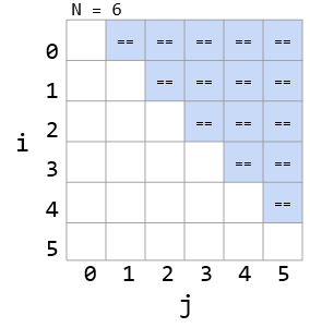
Worst case number of == operations:

C = 1 + 2 + 3 + … + (N - 3) + (N - 2) + (N - 1) = N(N - 1) / 2

• Given by area of right triangle of side length N-1.

• Order of growth of area is N^2.

Big-Theta

Formalizing Order of Growth

Given a function Q(N), we can apply our last two simplifications (ignore low orders terms and multiplicative constants) to yield the order of growth of Q(N).

• Example: Q(N) = 3N^3 + N^2

• Order of growth: N^3

Let’s finish out this lecture by moving to a more formal notation called Big-Theta.

• The math might seem daunting at first.

• … but the idea is exactly the same! Using “Big-Theta” instead of “order of growth” does not change the way we analyze code at all.

Big-Theta

Suppose we have a function R(N) with order of growth f(N).

• In “Big-Theta” notation we write this as R(N) ∈ Θ(f(N)).

• Examples:

  • N^3 + 3N^4 ∈ Θ(N^4)
  • 1/N + N3 ∈ Θ(N^3)
  • 1/N + 5 ∈ Θ(1)
  • Ne^N + N ∈ Θ(Ne^N)
  • 40sin(N) + 4N^2 ∈ Θ(N^2)

Big-Theta: Formal Definition

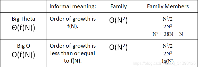
R(N) ∈ Θ(f(N)) means there exist positive constants k1 and k2 such that: k1f(N) <= R(N) <= k2f(N) for all values of N larger than some N0. (i.e. very large N)

We used Big Theta to describe the order of growth of a function.

We also used Big Theta to describe the rate of growth of the runtime of a piece of code.

Big O Notation

Whereas Big Theta can informally be thought of as something like “equals”, Big O can be thought of as “less than or equal”.

Example, the following are all true:

• N^3 + 3N^4 ∈ Θ(N^4)

• N^3 + 3N^4 ∈ O(N^4)

• N^3 + 3N^4 ∈ O(N^6)

• N^3 + 3N^4 ∈ O(N!)

• N^3 + 3N^4 ∈ O(N^N!)

Big O: Formal Definition

R(N) ∈ O(f(N)) means there exists positive constants k2 such that: R(N) <= k2f(N) for all values of N greater than some N0. (i.e. very large N)

Example: 40 sin(N) + 4N2 ∈ O(N4)

• R(N) = 40 sin(N) + 4N2

• f(N) = N4

• k2 = 1

Big Theta vs. Big O

We will see why big O is practically useful in the next lecture.

Summary

Given a code snippet, we can express its runtime as a function R(N), where N is some property of the input of the function (often the size of the input).

Rather than finding R(N) exactly, we instead usually only care about the order of growth of R(N).

One approach (not universal):

• Choose a representative operation, and let C(N) be the count of how many times that operation occurs as a function of N.

• Determine order of growth f(N) for C(N), i.e. C(N) ∈ Θ(f(N))

  • Often (but not always) we consider the worst case count.

• If operation takes constant time, then R(N) ∈ Θ(f(N))

• Can use O as an alternative for Θ. O is used for upper bounds.