


 本文探讨了渐进分析的基本概念,通过对比两种不同算法的复杂度,介绍了Big-Theta标记法及其在评估代码性能中的应用。文章详细分析了算法的运行时间和调用次数,展示了如何使用Python进行算法效率的实测,并引入了Big-Theta标记法来描述算法的复杂度。
渐进分析 Note
1. Introdiction
渐进分析 (Asymptotic Analysis)主要用于评估代码的性能
Old saying:
An engineer will do for a dim what any fool will do for a dollar.
垃圾的代码: 使用不合适的数据结构、复杂、缓慢、占用大量内存
好的代码:合适的数据结构、简洁、高效、使用合理的内存开销
2. Big-Theta Notation - Θ \Theta Θ
2.1 Example-Duplicate Detection
考虑分析在如下的列表中,查找出重复元素的两种方法的算法复杂度:
| -3 | -1 | 2 | 4 | 4 | 8 | 12 |
|---|
implimentation of comparing algorithm
Object: 查找array中是否存在重复的元素
Determine if their is any duplicates in the array。
一个基本的想法是考虑所有可能的情况
A silly method
def sillySearch(x):
	OperationCount = 0
	print('I compare every possible pair!')
	lengthOfX = len(x)
	for _ in range(lengthOfX):
		currentA = x[_]
		for i in range(_+1,lengthOfX):
			OperationCount +=1
			print("Comparing ",str(x[_])+"=="+str(x[i]),"Operation Count: ",str(OperationCount))
			if x[_]==x[i]:
				print(str(x[_])+"="+str(x[i]))
				return True
程序输出:
I compare every possible pair!
Comparing  -3==-1 Operation Count:  1
Comparing  -3==2 Operation Count:  2
Comparing  -3==4 Operation Count:  3
Comparing  -3==4 Operation Count:  4
Comparing  -3==8 Operation Count:  5
Comparing  -3==12 Operation Count:  6
Comparing  -1==2 Operation Count:  7
Comparing  -1==4 Operation Count:  8
Comparing  -1==4 Operation Count:  9
Comparing  -1==8 Operation Count:  10
Comparing  -1==12 Operation Count:  11
Comparing  2==4 Operation Count:  12
Comparing  2==4 Operation Count:  13
Comparing  2==8 Operation Count:  14
Comparing  2==12 Operation Count:  15
Comparing  4==4 Operation Count:  16
4=4
0:00:00.000192
[Finished in 1.9s]
一个更好的方法是只考虑相邻的情况
# a little bit cleverer method
# only consider the neighboring duplication
def betterSearch(x):
	OperationCount = 0
	print('I compare neighboring pairs!')
	lengthOfX = len(x)
	for _ in range(lengthOfX):
		currentA = x[_]
		OperationCount +=1
		print("Comparing ",str(x[_])+"=="+str(x[_+1]),"Operation Count: ",str(OperationCount))
		if x[_]==x[_+1]:
			print(str(x[_])+"="+str(x[_+1]))
			return True
程序输出:
I compare neighboring pairs!
Comparing  -3==-1 Operation Count:  1
Comparing  -1==2 Operation Count:  2
Comparing  2==4 Operation Count:  3
Comparing  4==4 Operation Count:  4
4=4
0:00:00.000059
[Finished in 1.7s]
记
n
n
n为比较(
=
=
==
==)的次数。
比较silly的baseline方法用了192个单位时间。
n
=
16
n=16
n=16
改进的方法用了59个单位时间.
n
=
4
n=4
n=4
where
n
n
n is the count of the operating steps
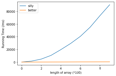
2.1.1 小实验(运行时间随规模增加的变化)
在最坏的情况下(把重复项放到数组x的末尾),两种查重算法的运行时间(ms)与数组
x
x
x的长度的关系。可见随着数组长度增加,silly方法的运行情况指数级恶化。
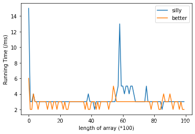
但是,在最好的情况下(数组中所有元素相同),二者的表现相差不大:
此时用x = [0]*N对数组x 进行初始化
测试并绘图使用的源代码如下:
# A silly method
def sillySearch(x):
	OperationCount = 0
	# print('I compare every possible pair!')
	lengthOfX = len(x)
	for _ in range(lengthOfX):
		currentA = x[_]
		for i in range(_+1,lengthOfX):
			OperationCount +=1
			# print("Comparing
			if x[_]==x[i]:
				return True

# a little bit cleverer method
# only consider the neighboring duplication
def betterSearch(x):
	OperationCount = 0
	# print('I compare neighboring pairs!')
	lengthOfX = len(x)
	for _ in range(lengthOfX-1):
		currentA = x[_]
		OperationCount +=1
		if x[_]==x[_+1]:
			# print(str(x[_])+"="+str(x[_+1]))
			return True

import datetime
from matplotlib import pyplot as plt
# x = [-3,-1,2,4,4,8,12]

sillyRecorder = []
betterRecorder = []
#test silly
for N in range(1,1000,100):
	x = list(range(0,N-1))
	x.append(N-2)
	start = datetime.datetime.now()
	sillySearch(x)
	    # do something
	end = datetime.datetime.now()
	sillyRecorder.append((end-start).microseconds)
for N in range(1,1000,100):
	x = list(range(0,N-1))
	x.append(N-2)
	start = datetime.datetime.now()
	betterSearch(x)
	end = datetime.datetime.now()
	betterRecorder.append((end-start).microseconds)

plt.plot(sillyRecorder)
plt.plot(betterRecorder)
plt.legend(['silly','better'])
plt.show()
plt.xlabel('length of array')
plt.xlabel('Running Time (/ms)')
print(sillyRecorder)
2.2一般描述算法复杂性的方法
为了描绘一个算法的复杂性,需要建立一种同时具有简单(simple)和数学严谨性(mathematically rigious)的描述方法,使得上述两种算法的复杂度一目了然。首先来看一下常见的描述算法性能的方法,然后逐渐过渡到Big-Theta Notation - Θ \Theta Θ。
2.2.1使用python计时器进行精确评估
1:对python文件的运行时间进行计时
在终端中输入:
>> time python 文件名
2: 对指定代码块的运行时间进行计时
import datetime
start = datetime.datetime.now()
代码块
end = datetime.datetime.now()
print (end-start)
2.2.2 计算代码中每一步的调用次数
考虑到算法规模为
N
N
N的情况(即待查找的list长度为
N
N
N),
对于比较“笨”的这种算法:
def sillySearch(x):
	lengthOfX = len(x)
	for _ in range(lengthOfX):
		currentA = x[_]
		for i in range(_+1,lengthOfX):
			OperationCount +=1
			if x[_]==x[i]:
				print(str(x[_])+"="+str(x[i]))
				return True
各个功能块的执行次数、最好的情况到最差的情况如下:
| Operation | Count |
|---|---|
| range calls | 2 to N + 1 N+1 N+1 |
| len calls | 2 to N + 1 N+1 N+1 |
| _ assignments | 1 to N − 1 N-1 N−1 |
| j assignments | 1 to N 2 − N 2 \frac{N^2-N}{2} 2N2−N |
| equals(==) | 1 to N 2 − N 2 \frac{N^2-N}{2} 2N2−N |
| array access) | 2 to N 2 − N N^2-N N2−N |
对于比较聪明的算法:
# a little bit cleverer method
# only consider the neighboring duplication
def betterSearch(x):
	OperationCount = 0
	lengthOfX = len(x)
	for _ in range(lengthOfX):
		currentA = x[_]
		OperationCount +=1
		if x[_]==x[_+1]:
			return True
各个功能块的执行次数、最好的情况到最差的情况如下:
| Operation | Count |
|---|---|
| range calls | 1 |
| len calls | 1 |
| _ assignments | 1 to N − 1 N-1 N−1 |
| equals(==) | 1 to N − 1 N-1 N−1 |
| array access) | 2 to 2 N − 2 2N-2 2N−2 |
2.2.2.1 对“调用次数”指标进行简化
我们可以依据以下规则对上述的评估方式进行适当简化:
- 只考虑最差的情况(Only consider the worst case)
- 选择具有代表性的操作(Representative Operation)
- 忽略低次项(Ignore lower order terms)
- 忽略乘法计算的常系数 (Ignore multiplicative constant)
假设说有这么一个算法的操作计数表:
| Operation | Count |
|---|---|
| Op_1 | 1 |
| Op_2 | 1 to N N N |
| Op_3 | 1 to N 2 − N 2 \frac{N^2-N}{2} 2N2−N |
| Op_4 | 0 to N 2 + 3 N + 2 2 \frac{N^2+3N+2}{2} 2N2+3N+2 |
这个表可以被进一步简化为:
| Operation | Count |
|---|---|
| Op_3 | N 2 N^2 N2 |
于是现在就有以一种基于数学假设的更严谨的方式,使用 N 2 N^2 N2来刻画这个算法的复杂度。
实际上一个算法的复杂度取决于最最糟糕的情况下,操作复杂度增长的数量级。
2.3 Big theta- Θ \Theta Θ
-Example:
Q
(
N
)
=
3
N
3
+
N
2
Q(N)=3N^3+N^2
Q(N)=3N3+N2
-Order of growth:
N
3
N^3
N3
| function | Order of growth |
|---|---|
| N 3 + 3 N 4 N^3+3N^4 N3+3N4 | N 4 N^4 N4 |
| 1 N + N 3 \frac{1}{N}+N^3 N1+N3 | N 3 N^3 N3 |
| 1 N + 5 \frac{1}{N}+5 N1+5 | 1 |
| N e N + N Ne^N+N NeN+N | N e N Ne^N NeN |
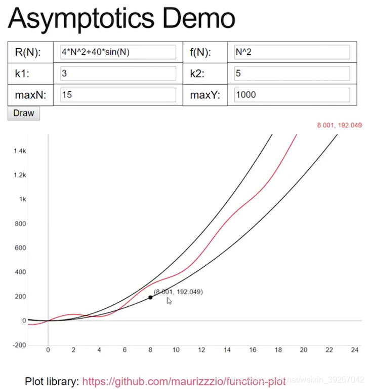
| 40 ∗ s i n ( N ) + 4 N 2 40*sin(N)+4N^2 40∗sin(N)+4N2 | N 2 N^2 N2 |
Big-Theta的定义:
假设我们有一个函数
R
(
N
)
R(N)
R(N),有一个增长的order
f
(
N
)
f(N)
f(N)(order of growth)。
在“Big-Theta” 的标记方式里,我们把这个关系写为:
R
(
N
)
∈
Θ
(
f
(
N
)
)
R(N)\in \Theta(f(N))
R(N)∈Θ(f(N))
例如:
- N 3 + 3 N 4 ∈ Θ ( N 4 ) N^3+3N^4\in\Theta(N^4) N3+3N4∈Θ(N4)
- 1 N + N 3 ∈ Θ ( N 3 ) \frac{1}{N}+N^3\in \Theta(N^3) N1+N3∈Θ(N3)
- 1 N + 5 ∈ Θ ( 1 ) \frac{1}{N}+5\in\Theta(1) N1+5∈Θ(1)
- N e N + N ∈ Θ ( N e N ) Ne^N+N\in\Theta(Ne^N) NeN+N∈Θ(NeN)
-
40
∗
s
i
n
(
N
)
+
4
N
2
∈
Θ
(
N
2
)
40*sin(N)+4N^2\in\Theta(N^2)
40∗sin(N)+4N2∈Θ(N2)
注意,有的情况下,有人会选择将上述的 ∈ \in ∈换成 = = =。
更具体而言,当我们说
R
(
N
)
∈
Θ
(
f
(
N
)
)
R(N)\in \Theta(f(N))
R(N)∈Θ(f(N))的时候,等价于存在两个为正的常数
k
1
k_1
k1和
k
2
k_2
k2, 于是有:
k
1
⋅
f
(
N
)
≤
R
(
N
)
≤
k
2
⋅
f
(
N
)
k_1\cdot f(N)\leq R(N)\leq k_2\cdot f(N)
k1⋅f(N)≤R(N)≤k2⋅f(N)
对于所有的
N
N
N当
N
0
≤
N
N_0 \leq N
N0≤N时成立


 403
403

 被折叠的 条评论
为什么被折叠?
被折叠的 条评论
为什么被折叠?
 到【灌水乐园】发言


