BIOS14:Statistic Exercise 2

a) Does the treatment (added mice) affect the relationship between habitat quality and elephant density? (5p)

Firstly, I checked the data and found that there is a clear linear relationship between elephant density and plants quality without mice added. But in the treatment, the elephant density a appears different degree of decline after the mice added.

# data import and check
elemice = read.csv('elemice.csv')
str(elemice)
elemice_c = subset(elemice, treat == 'Control')
elemice_m = subset(elemice, treat == 'Mice added')
plot(eledens~plants, data=elemice_c, col = 'red')
points(eledens~plants, data=elemice_m, col = 'blue')
legend("topleft",  c("control","treatment"), pch = c(1,1), col=c("red", "blue"))

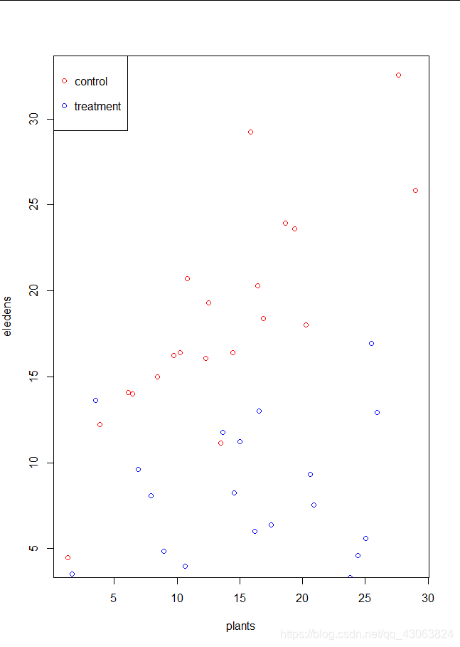
But from the scatter plot, there are some obviously multivariate outliers among red points.

Then construct linear model

# Construct mode
fit = lm(eledens~plants, data=elemice_c)

Check assumptions

# No autocorrelation
> dwtest(fit)

	Durbin-Watson test

data:  fit
DW = 2.2368, p-value = 0.7186
alternative hypothesis: true autocorrelation is greater than 0

# The residuals from the regression are normally distributed
> shapiro.test(fit$residuals)

	Shapiro-Wilk normality test

data:  fit$residuals
W = 0.95494, p-value = 0.4483

> x <-fit$residuals
> y <-pnorm(summary(x), mean =mean(x, na.rm=TRUE), sd =sd(x, na.rm=TRUE))
> ks.test(x, y)

	Two-sample Kolmogorov-Smirnov test

data:  x and y
D = 0.4, p-value = 0.3713
alternative hypothesis: two-sided

par(mfrow=c(2,2))
plot(fit)
par(mfrow=c(1,1))

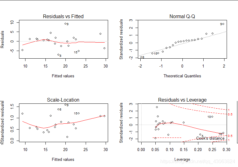
The red fit line for the scale-location plot and residuals-fitted plot is a bit all over the place, this is probably mainly because there are few multivariate outliers.

#Regression results
> anova(fit)
Analysis of Variance Table

Response: eledens
          Df Sum Sq Mean Sq F value   Pr(>F)    
plants     1 531.44  531.44  36.586 1.02e-05 ***
Residuals 18 261.47   14.53                     
---
Signif. codes:  0 ‘***’ 0.001 ‘**’ 0.01 ‘*’ 0.05 ‘.’ 0.1 ‘ ’ 1
> summary(fit)

Call:
lm(formula = eledens ~ plants, data = elemice_c)

Residuals:
    Min      1Q  Median      3Q     Max 
-7.1022 -2.4141  0.6333  1.3977  9.2354 

Coefficients:
            Estimate Std. Error t value Pr(>|t|)    
(Intercept)   8.3028     1.8732   4.433 0.000321 ***
plants        0.7368     0.1218   6.049 1.02e-05 ***
---
Signif. codes:  0 ‘***’ 0.001 ‘**’ 0.01 ‘*’ 0.05 ‘.’ 0.1 ‘ ’ 1

Residual standard error: 3.811 on 18 degrees of freedom
Multiple R-squared:  0.6702,	Adjusted R-squared:  0.6519 
F-statistic: 36.59 on 1 and 18 DF,  p-value: 1.02e-05

The anova gives a significant result, which means there is a linear relationship between two variables.

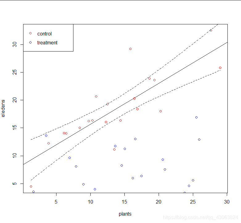
b) Illustrate your findings in a) with a graph. If appropriate, include some sort of fitted line(s) or predicted values. Motivate your decision. (2p)

# Illustrate the result
plot(eledens~plants, data=elemice_c,  pch=1, col="red")
abline(fit)
new.x = seq(min(elemice_c$plants), max(elemice_c$plants), len=100)
pred = predict(fit, new=data.frame(plants=new.x), interval="conf")
lines(new.x,pred[,"lwr"],lty=2)
lines(new.x,pred[,"upr"],lty=2)
points(eledens~plants, data=elemice_m, col = 'blue')
legend("topleft",  c("control","treatment"), pch = c(1,1), col=c("red", "blue"))

c) Write out the equations for the model you found best describing the data in a). What conclusions can you draw when looking at the confidence intervals for the parameters.? (3p)

The model I found is:
$$\begin{gathered} y=0.7368x+8.3028 \\ y:elephantsdensity \\ x:plantsquality \end{gathered}$$
From the figure in b), we can see most of blue points(the treatment) is out of the confidence intervals which means the mice added does have effect on the relationship between elephants density and plants quality. In other words, the elephants truly afraid of mice.