机器学习（1）关系拟合（回归）与区分类型（分类）

这波全新的学习遭老罪了，几乎啥都看不明白，一个一个查，感觉注释有代码两倍长。

一、回归

import torch
import torch.nn.functional as F
import matplotlib.pyplot as plt

#-----建立数据集-----


# torch.manual_seed(1)    # reproducible可再生的

x = torch.unsqueeze(torch.linspace(-1, 1, 100), dim=1)  # x data (tensor), shape=(100, 1)
#numpy.linspace 函数用于创建一个一维数组，数组是一个等差数列构成的，格式如下：
#unsqueeze用来增加张量，torch中只能处理二维信息，在指定位置 dim 插入一个大小为1的维度

y = x.pow(2) + 0.2*torch.rand(x.size())                 # noisy y data (tensor), shape=(100, 1)
#这一行的意思是把y和x相关，添加噪点

# torch can only train on Variable, so convert them to Variable
# The code below is deprecated in Pytorch 0.4. Now, autograd directly supports tensors
# x, y = Variable(x), Variable(y)

# plt.scatter(x.data.numpy(), y.data.numpy())
# plt.show()

#-----建立神经网络-----

class Net(torch.nn.Module):    #继承torch的组件
    #class(类)是面向对象编程的基本概念，是一种自定义数据结构类型 命名为Net

    #init搭建这个信息层所需要的信息
    def __init__(self, n_feature, n_hidden, n_output):
        super(Net, self).__init__()    # 继承 __init__ 功能
        #首先找到Net的父类（比如是类nn.Module），然后把类Net的对象self转换为类nn.Module的对象，然后“被转换”的类nn.Module对象调用自己的init函数
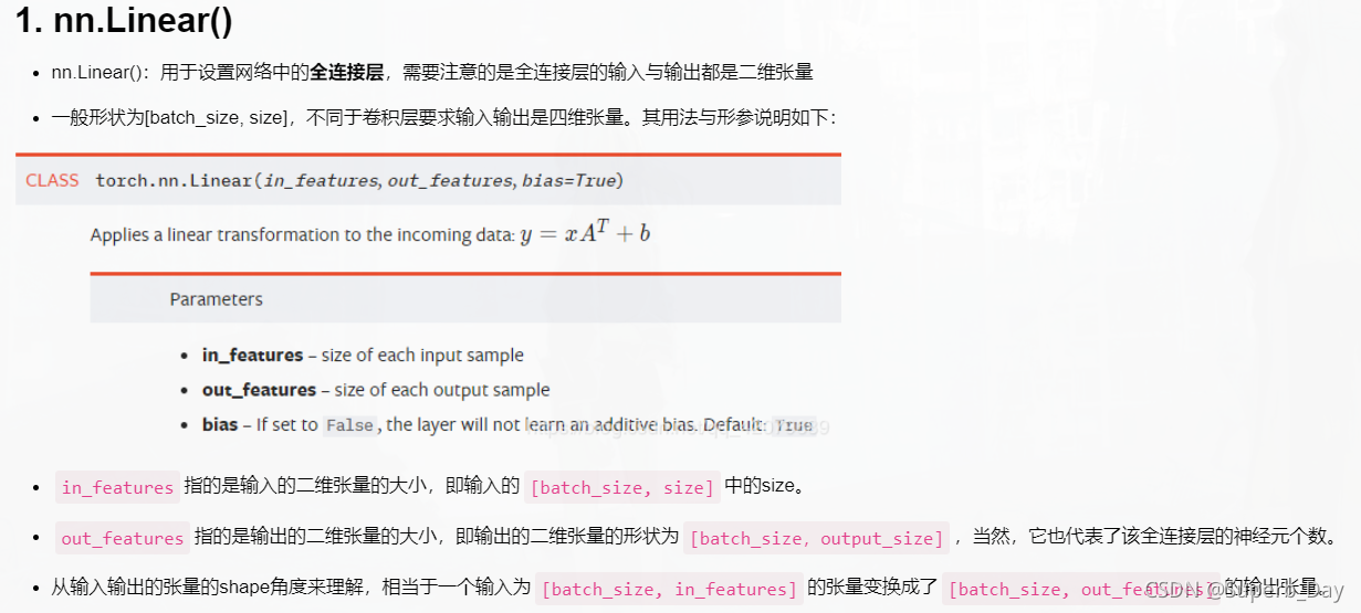
        self.hidden = torch.nn.Linear(n_feature, n_hidden)   # 隐藏层线性输出
        self.predict = torch.nn.Linear(n_hidden, n_output)   # 输出层线性输出
        #nn.Linear()：用于设置网络中的全连接层，需要注意的是全连接层的输入与输出都是二维张量
        #【此处注释一】#

    #把前面的内容一个一个传递到这里进行组合，搭流程图就是forward所做的事情。
    def forward(self, x): #x为输入信息
        # 正向传播输入值, 神经网络分析出输出值
        x = F.relu(self.hidden(x))      # activation function for hidden layer
        #relu是小于0的改为0，大于0的不管的激励函数
        x = self.predict(x)             # linear output
        #此步骤用来输出
        return x

net = Net(n_feature=1, n_hidden=10, n_output=1)     # define the network
#输入值1个，神经元10个，输出1个。
print(net)  # net architecture
"""
Net (
  (hidden): Linear (1 -> 10)
  #此处意思为hidden linear 从一个输入到10个神经元
  (predict): Linear (10 -> 1)
  #此处意思为hidden linear 从10个神经元输出一个
)
"""

#-----此处为训练网络-----

# optimizer 是训练的工具
optimizer = torch.optim.SGD(net.parameters(), lr=0.2)
#torch.optim.SGD()是个优化器，传入神经网络参数net.parameters(),lr：learning rate，学习效率
loss_func = torch.nn.MSELoss()  # this is for regression mean squared loss
#loss_func 计算误差的一种手段，torch.nn.MSELoss()是均方差



plt.ion()   # something about plotting
#设置为实时打印的过程



#-----训练开始-----

for t in range(200): #训练200步
    prediction = net(x)     # input x and predict based on x
    #把输入信息放进去得到输出

    loss = loss_func(prediction, y)     # must be (1. nn output, 2. target)
    #实际输出值和预测值的误差大小

    #这三步为优化步骤
    optimizer.zero_grad()   # clear gradients for next train
    #将梯度将为0，因为每一次计算loss以后，梯度都会保留在net里面
    loss.backward()         # backpropagation, compute gradients
    #反向传播，计算出节点中的梯度
    optimizer.step()        # apply gradients
    #以上面的learning rate 0.2 来优化梯度

#-----以下为可视化-----
#每学习5步打印一次
    if t % 5 == 0:
        # plot and show learning process
        plt.cla()
        plt.scatter(x.data.numpy(), y.data.numpy())
        plt.plot(x.data.numpy(), prediction.data.numpy(), 'r-', lw=5)
        plt.text(0.5, 0, 'Loss=%.4f' % loss.data.numpy(), fontdict={'size': 20, 'color':  'red'})
        plt.pause(0.1)

plt.ioff()
plt.show()

注释1：

二、分类

import torch
import torch.nn.functional as F
import matplotlib.pyplot as plt

#-----建立数据集-----


# torch.manual_seed(1)    # reproducible可再生的

x = torch.unsqueeze(torch.linspace(-1, 1, 100), dim=1)  # x data (tensor), shape=(100, 1)
#numpy.linspace 函数用于创建一个一维数组，数组是一个等差数列构成的，格式如下：
#unsqueeze用来增加张量，torch中只能处理二维信息，在指定位置 dim 插入一个大小为1的维度

y = x.pow(2) + 0.2*torch.rand(x.size())                 # noisy y data (tensor), shape=(100, 1)
#这一行的意思是把y和x相关，添加噪点

# torch can only train on Variable, so convert them to Variable
# The code below is deprecated in Pytorch 0.4. Now, autograd directly supports tensors
# x, y = Variable(x), Variable(y)

# plt.scatter(x.data.numpy(), y.data.numpy())
# plt.show()

#-----建立神经网络-----

class Net(torch.nn.Module):    #继承torch的组件
    #class(类)是面向对象编程的基本概念，是一种自定义数据结构类型 命名为Net

    #init搭建这个信息层所需要的信息
    def __init__(self, n_feature, n_hidden, n_output):
        super(Net, self).__init__()    # 继承 __init__ 功能
        #首先找到Net的父类（比如是类nn.Module），然后把类Net的对象self转换为类nn.Module的对象，然后“被转换”的类nn.Module对象调用自己的init函数
        self.hidden = torch.nn.Linear(n_feature, n_hidden)   # 隐藏层线性输出
        self.predict = torch.nn.Linear(n_hidden, n_output)   # 输出层线性输出
        #nn.Linear()：用于设置网络中的全连接层，需要注意的是全连接层的输入与输出都是二维张量
        #【此处注释一】#

    #把前面的内容一个一个传递到这里进行组合，搭流程图就是forward所做的事情。
    def forward(self, x): #x为输入信息
        # 正向传播输入值, 神经网络分析出输出值
        x = F.relu(self.hidden(x))      # activation function for hidden layer
        #relu是小于0的改为0，大于0的不管的激励函数
        x = self.predict(x)             # linear output
        #此步骤用来输出
        return x

net = Net(n_feature=1, n_hidden=10, n_output=1)     # define the network
#输入值1个，神经元10个，输出1个。
print(net)  # net architecture
"""
Net (
  (hidden): Linear (1 -> 10)
  #此处意思为hidden linear 从一个输入到10个神经元
  (predict): Linear (10 -> 1)
  #此处意思为hidden linear 从10个神经元输出一个
)
"""

#-----此处为训练网络-----

# optimizer 是训练的工具
optimizer = torch.optim.SGD(net.parameters(), lr=0.2)
#torch.optim.SGD()是个优化器，传入神经网络参数net.parameters(),lr：learning rate，学习效率
loss_func = torch.nn.MSELoss()  # this is for regression mean squared loss
#loss_func 计算误差的一种手段，torch.nn.MSELoss()是均方差



plt.ion()   # something about plotting
#设置为实时打印的过程



#-----训练开始-----

for t in range(200): #训练200步
    prediction = net(x)     # input x and predict based on x
    #把输入信息放进去得到输出

    loss = loss_func(prediction, y)     # must be (1. nn output, 2. target)
    #实际输出值和预测值的误差大小

    #这三步为优化步骤
    optimizer.zero_grad()   # clear gradients for next train
    #将梯度将为0，因为每一次计算loss以后，梯度都会保留在net里面
    loss.backward()         # backpropagation, compute gradients
    #反向传播，计算出节点中的梯度
    optimizer.step()        # apply gradients
    #以上面的learning rate 0.2 来优化梯度

#-----以下为可视化-----
#每学习5步打印一次
    if t % 5 == 0:
        # plot and show learning process
        plt.cla()
        plt.scatter(x.data.numpy(), y.data.numpy())
        plt.plot(x.data.numpy(), prediction.data.numpy(), 'r-', lw=5)
        plt.text(0.5, 0, 'Loss=%.4f' % loss.data.numpy(), fontdict={'size': 20, 'color':  'red'})
        plt.pause(0.1)

plt.ioff()
plt.show()