14-降噪自编码-增强抗干扰能力

一、前言
本篇将围绕TinyMind 汉字书法识别自由练习赛中的比赛数据中单个字做数据增强操作，就是依据降噪自编码的原理将相对标准的字形作为训练结果，然后将比赛的单个字所有数据作为输入，简单训练一个有回溯能力的网络结构。该结构近似的将比赛数据模拟成噪声数据，输出的结果为真实的数据，这样可以在更多分类任务时让模型拥有更好的鲁棒性。也就会获得更好的结果。
二、相关概念
去噪自编码器：（Denoising Autoencoder，DA），是在自动编码的基础上，训练数据加入噪声，输出的标签仍是原始的样本（没有加过噪声的）,这样自动编码器必须学习去除噪声而获得真正的没有被噪声污染过的输入特征。因此，这就迫使编码器去学习输入信号的更加鲁棒的特征表达，即具有更好的泛化能力。
三、具体实现
本篇只显示关键代码字段

#获取去噪编码结果
def get_Y(size=(64,64),channels=1):
    #list_words=os.listdir('words')
    #读取图片信息
    word_name='且.png'
    file_content=tf.gfile.FastGFile('words/'+word_name,'rb').read()
    #解码
    image_tensor=tf.image.decode_png(file_content,channels=channels)
    #resize image
    image_tensor=tf.image.resize_images(image_tensor,size=size,method=tf.image.ResizeMethod.NEAREST_NEIGHBOR)

    image_tensor=tf.reshape(image_tensor,[-1,4096])
    print(image_tensor.get_shape())
    return image_tensor

#学习参数
weight={
    'h1':tf.Variable(tf.random_normal([n_input,n_hidden_1])),
    'h2':tf.Variable(tf.random_normal([n_hidden_1,n_hidden_1])),
    'out':tf.Variable(tf.random_normal([n_hidden_1,n_input]))
}
biases={
    'b1':tf.Variable(tf.zeros([n_hidden_1])),
    'b2':tf.Variable(tf.zeros([n_hidden_1])),
    'out':tf.Variable(tf.zeros([n_input]))
}

#网络模型
def encoder(X_input,weight,biases):
    layer_1=tf.nn.sigmoid(tf.add(tf.matmul(X_input,weight['h1']),biases['b1']))
    #layer_1out=tf.nn.dropout(layer_1,keep_prob=1)
    layer_2=tf.nn.sigmoid(tf.add(tf.matmul(layer_1,weight['h2']),biases['b2']))
    #layer_2out=tf.nn.dropout(layer_2,keep_prob=1)
    return tf.matmul(layer_2,weight['out'])+biases['out']

tf.InteractiveSession()
#获取数据
train_X=read_train_data.get_a_category_message('且')   #(400,4096)
train_Y=get_Y()                        #(1,4096)
train_Y=train_Y.eval()
#定义占位符
X=tf.placeholder(tf.float32,[None,4096])
Y=tf.placeholder(tf.float32,[None,4096])

reconstruction=encoder(X,weight,biases)
#损失函数计算
cost=tf.reduce_mean(tf.pow(reconstruction-Y,2))
#优化器优化
#optm=tf.train.AdamOptimizer(learning_rate=0.01).minimize(cost)
optm=tf.train.GradientDescentOptimizer(learning_rate=0.01).minimize(cost)

#训练模型
def train():
    train_epochs = 3000
    batch_size = 1
    display_step=20
    save_epoch_num=30

    with tf.Session() as sess:
        #变量初始化
        sess.run(tf.global_variables_initializer())
        print('开始训练\n')
        # 定义模型保存对象
        saver = tf.train.Saver()
        # 重载保存的中间模型
        result = [0]
        # 查看模型状态
        ckpt = tf.train.get_checkpoint_state('./model')
        # 加载模型
        if ckpt and ckpt.model_checkpoint_path:
            print("model restoring")
            saver.restore(sess, ckpt.model_checkpoint_path)
            print(ckpt.model_checkpoint_path)
            pattern = re.compile('\d+')
            result = pattern.findall(ckpt.model_checkpoint_path)
            print(result[0])
        #显示结果
        for item in range(40):
            tmp_X=np.reshape(train_X[item*10:(item+1)*10],[-1,4096])
            feeds={X:tmp_X}
            encode_decode=sess.run(reconstruction,feed_dict=feeds)
            #创建子图
            f,a=plt.subplots(3,10,figsize=(10,3))
            for i in range(10):
                a[0][i].imshow(np.reshape(tmp_X[i],(64,64)),cmap=plt.get_cmap('gray'))
                a[1][i].imshow(np.reshape(encode_decode[i],(64,64)),cmap=plt.get_cmap('gray'))
                a[2][i].imshow(np.reshape(train_Y,(64,64)),cmap=plt.get_cmap('gray'))
            plt.show()
        # for epoch in range(train_epochs-int(result[0])):
        #
        #     # 400为训练集条数
        #     index = np.random.permutation(400)
        #     total_cost=0
        #     for item in range(400):
        #         #获取训练集索引信息
        #         train_index=index[item]
        #         #训练模型
        #         tmp_X=np.reshape(train_X[train_index],[-1,4096])
        #         feeds={X:tmp_X,Y:train_Y}
        #         sess.run(optm,feed_dict=feeds)
        #         cost_=sess.run(cost,feed_dict=feeds)
        #         total_cost+=cost_
        #
        #         #if item%display_step==0:
        #             #print("epoch:{},step:{},loss:{}".format(epoch+1,item+1,cost_))
        #     print("epoch:{}  average cost: {}".format(epoch + 1+int(result[0]), total_cost/400))
        #     if (epoch+1)%save_epoch_num==0:
        #         #.ckpt模型保存
        #         saver.save(sess,'./model/model',global_step=epoch+1+int(result[0]))
        #         print("{} model had saved in ./model/model".format(epoch+1+int(result[0])))
        print("Finished!")

if __name__ =='__main__':

    train()

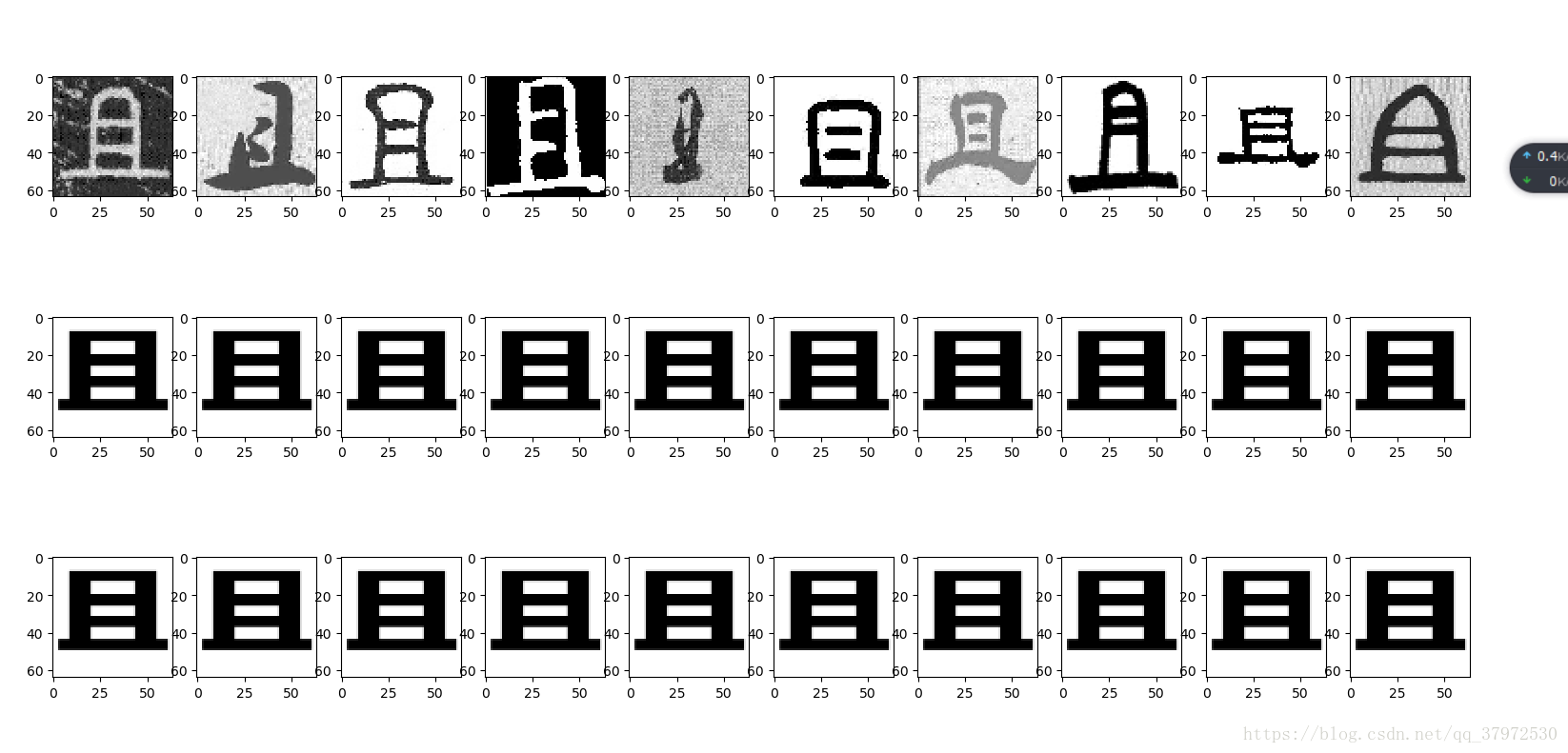
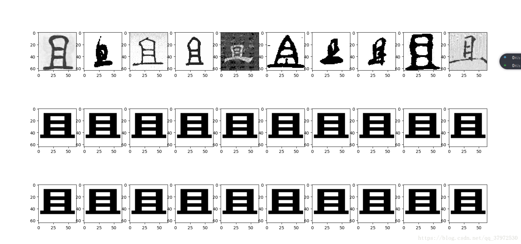
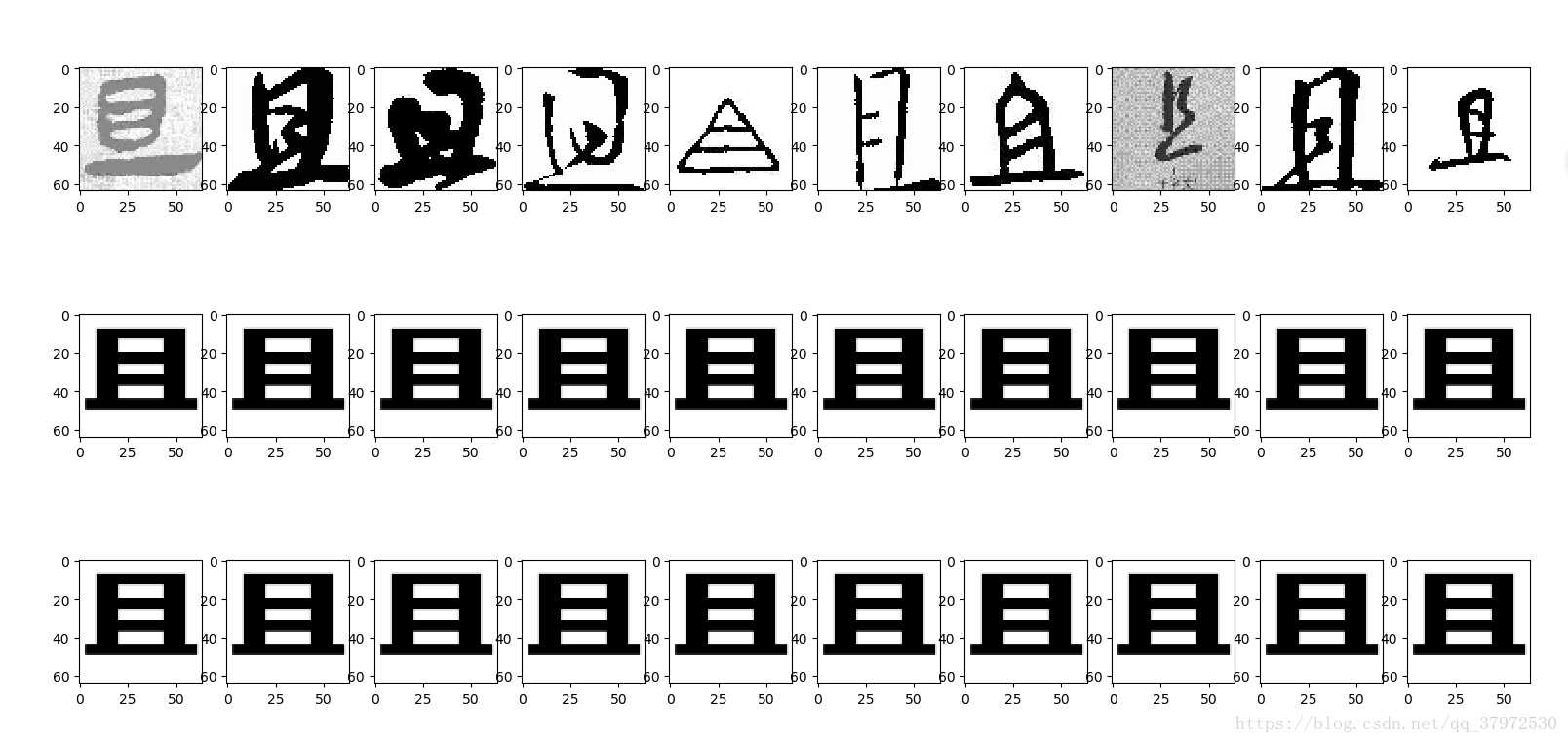
四、效果展示



五、分析与总结
如图所展示的几张图片，第一行是训练之前的数据，第二行是模型所计算的数据，第三行是目标数据，从效果上来看几乎看不出来区别，所以训练的结果还是比较好的。
拥有这样的训练结果，这跟数据量小的因素有绝大部分关系，总共400张图片所以模型的拟合能力和收敛能力都比较强，但是在后续的工作中还有更多的挑战要做。如有可能，后续的进度会更新至后面的博客中，敬请期待。