


 本研究深入分析了自行车共享需求的预测模型,利用历史数据探讨了季节、天气、工作日等因素对需求的影响,并通过多种机器学习算法进行模型训练,包括线性回归、岭回归、Lasso回归和梯度提升等,旨在提高预测精度。
import pylab
import calendar
import numpy as np
import pandas as pd
import seaborn as sn
from scipy import stats
import missingno as msno
from datetime import datetime
import matplotlib.pyplot as plt
import warnings
pd.options.mode.chained_assignment = None
warnings.filterwarnings("ignore", category=DeprecationWarning)
%matplotlib inline
In [2]:
dailyData = pd.read_csv("C:/Users/_lc/BikeSharingDemand/train.csv")
dailyData.head(2)
Out[2]:
| datetime | season | holiday | workingday | weather | temp | atemp | humidity | windspeed | casual | registered | count | |
|---|---|---|---|---|---|---|---|---|---|---|---|---|
| 0 | 2011-01-01 00:00:00 | 1 | 0 | 0 | 1 | 9.84 | 14.395 | 81 | 0.0 | 3 | 13 | 16 |
| 1 | 2011-01-01 01:00:00 | 1 | 0 | 0 | 1 | 9.02 | 13.635 | 80 | 0.0 | 8 | 32 | 40 |
Out[58]:
| time | day | |
|---|---|---|
| 0 | 2011-01-01 00:00:00 | 1 |
| 1 | 2011-01-01 01:00:00 | 1 |
| 2 | 2011-01-01 02:00:00 | 1 |
| 3 | 2011-01-01 03:00:00 | 1 |
| 4 | 2011-01-01 04:00:00 | 1 |
In [5]:
datetime - hourly date + timestamp
season - 1 = spring, 2 = summer, 3 = fall, 4 = winter
holiday - whether the day is considered a holiday
workingday - whether the day is neither a weekend nor holiday
weather -
1: Clear, Few clouds, Partly cloudy, Partly cloudy
2: Mist + Cloudy, Mist + Broken clouds, Mist + Few clouds, Mist
3: Light Snow, Light Rain + Thunderstorm + Scattered clouds, Light Rain + Scattered clouds
4: Heavy Rain + Ice Pallets + Thunderstorm + Mist, Snow + Fog
temp - temperature in Celsius
atemp - "feels like" temperature in Celsius
humidity - relative humidity
windspeed - wind speed
casual - number of non-registered user rentals initiated
registered - number of registered user rentals initiated
count - number of total rentals (Dependent Variable)

dailyData.info()
<class 'pandas.core.frame.DataFrame'>
RangeIndex: 10886 entries, 0 to 10885
Data columns (total 12 columns):
datetime      10886 non-null object
season        10886 non-null int64
holiday       10886 non-null int64
workingday    10886 non-null int64
weather       10886 non-null int64
temp          10886 non-null float64
atemp         10886 non-null float64
humidity      10886 non-null int64
windspeed     10886 non-null float64
casual        10886 non-null int64
registered    10886 non-null int64
count         10886 non-null int64
dtypes: float64(3), int64(8), object(1)
memory usage: 1020.6+ KB
In [3]:
dailyData['date'] = dailyData['datetime'].map(lambda x: x.split()[0])
dailyData['datetime'] = pd.to_datetime(dailyData.datetime)
dailyData['month'] = dailyData['datetime'].map(lambda x: x.month)
dailyData['day'] = dailyData['datetime'].map(lambda x: x.day)
dailyData['hour'] = dailyData['datetime'].map(lambda x: x.hour)
dailyData['weekday'] = dailyData['datetime'].map(lambda x: x.weekday())
dailyData.head(2)
Out[3]:
| datetime | season | holiday | workingday | weather | temp | atemp | humidity | windspeed | casual | registered | count | date | month | day | hour | weekday | |
|---|---|---|---|---|---|---|---|---|---|---|---|---|---|---|---|---|---|
| 0 | 2011-01-01 00:00:00 | 1 | 0 | 0 | 1 | 9.84 | 14.395 | 81 | 0.0 | 3 | 13 | 16 | 2011-01-01 | 1 | 1 | 0 | 5 |
| 1 | 2011-01-01 01:00:00 | 1 | 0 | 0 | 1 | 9.02 | 13.635 | 80 | 0.0 | 8 | 32 | 40 | 2011-01-01 | 1 | 1 | 1 | 5 |
In [4]:
dailyData["season"] = dailyData.season.map({1: "Spring", 2 : "Summer", 3 : "Fall", 4 :"Winter" })
dailyData["weather"] = dailyData.weather.map({1: " Clear + Few clouds + Partly cloudy + Partly cloudy",\
                                        2 : " Mist + Cloudy, Mist + Broken clouds, Mist + Few clouds, Mist ", \
                                        3 : " Light Snow, Light Rain + Thunderstorm + Scattered clouds, Light Rain + Scattered clouds", \
                                        4 :" Heavy Rain + Ice Pallets + Thunderstorm + Mist, Snow + Fog " })
dailyData.head(2)
Out[4]:
| datetime | season | holiday | workingday | weather | temp | atemp | humidity | windspeed | casual | registered | count | date | month | day | hour | weekday | |
|---|---|---|---|---|---|---|---|---|---|---|---|---|---|---|---|---|---|
| 0 | 2011-01-01 00:00:00 | Spring | 0 | 0 | Clear + Few clouds + Partly cloudy + Partly c... | 9.84 | 14.395 | 81 | 0.0 | 3 | 13 | 16 | 2011-01-01 | 1 | 1 | 0 | 5 |
| 1 | 2011-01-01 01:00:00 | Spring | 0 | 0 | Clear + Few clouds + Partly cloudy + Partly c... | 9.02 | 13.635 | 80 | 0.0 | 8 | 32 | 40 | 2011-01-01 | 1 | 1 | 1 | 5 |
In [5]:
categoryVariableList = ["hour","weekday","month","season","weather","holiday","workingday"]
for var in categoryVariableList:
    dailyData[var] = dailyData[var].astype("category")
dailyData.head(2)
Out[5]:
| datetime | season | holiday | workingday | weather | temp | atemp | humidity | windspeed | casual | registered | count | date | month | day | hour | weekday | |
|---|---|---|---|---|---|---|---|---|---|---|---|---|---|---|---|---|---|
| 0 | 2011-01-01 00:00:00 | Spring | 0 | 0 | Clear + Few clouds + Partly cloudy + Partly c... | 9.84 | 14.395 | 81 | 0.0 | 3 | 13 | 16 | 2011-01-01 | 1 | 1 | 0 | 5 |
| 1 | 2011-01-01 01:00:00 | Spring | 0 | 0 | Clear + Few clouds + Partly cloudy + Partly c... | 9.02 | 13.635 | 80 | 0.0 | 8 | 32 | 40 | 2011-01-01 | 1 | 1 | 1 | 5 |
In [6]:
dailyData.drop('datetime', axis=1, inplace=True)
dailyData.head(2)
Out[6]:
| season | holiday | workingday | weather | temp | atemp | humidity | windspeed | casual | registered | count | date | month | day | hour | weekday | |
|---|---|---|---|---|---|---|---|---|---|---|---|---|---|---|---|---|
| 0 | Spring | 0 | 0 | Clear + Few clouds + Partly cloudy + Partly c... | 9.84 | 14.395 | 81 | 0.0 | 3 | 13 | 16 | 2011-01-01 | 1 | 1 | 0 | 5 |
| 1 | Spring | 0 | 0 | Clear + Few clouds + Partly cloudy + Partly c... | 9.02 | 13.635 | 80 | 0.0 | 8 | 32 | 40 | 2011-01-01 | 1 | 1 | 1 | 5 |
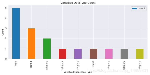
In [7]:
dataTypeDf = dailyData.dtypes.value_counts().to_frame().reset_index().rename(columns={'index':'variableType', 0:'count'})
sn.set_style('darkgrid')
ax = plt.figure(figsize=(10,4)).add_subplot(111)
dataTypeDf.plot(kind='bar',x="variableType",y="count",ax=ax)
ax.set(xlabel='variableTypeariable Type', ylabel='Count',title="Variables DataType Count")
Out[7]:
[Text(0, 0.5, 'Count'),
 Text(0.5, 0, 'variableTypeariable Type'),
 Text(0.5, 1.0, 'Variables DataType Count')]
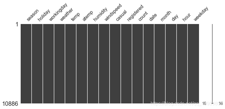
In [8]:
msno.matrix(dailyData,figsize=(12,5))
Out[8]:
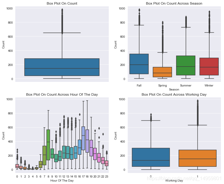
In [8]:
fig, axes = plt.subplots(nrows=2,ncols=2)
fig.set_size_inches(12, 10)
sn.boxplot(data=dailyData,y="count",orient="v",ax=axes[0][0])
sn.boxplot(data=dailyData,y="count",x="season",orient="v",ax=axes[0][1])
sn.boxplot(data=dailyData,y="count",x="hour",orient="v",ax=axes[1][0])
sn.boxplot(data=dailyData,y="count",x="workingday",orient="v",ax=axes[1][1])

axes[0][0].set(ylabel='Count',title="Box Plot On Count")
axes[0][1].set(xlabel='Season', ylabel='Count',title="Box Plot On Count Across Season")
axes[1][0].set(xlabel='Hour Of The Day', ylabel='Count',title="Box Plot On Count Across Hour Of The Day")
axes[1][1].set(xlabel='Working Day', ylabel='Count',title="Box Plot On Count Across Working Day")
Out[8]:
[Text(0, 0.5, 'Count'),
 Text(0.5, 0, 'Working Day'),
 Text(0.5, 1.0, 'Box Plot On Count Across Working Day')]
In [9]:
dailyDataWithoutOutliers = dailyData[np.abs(dailyData["count"]-dailyData["count"].mean())<=(3*dailyData["count"].std())]
len(dailyDataWithoutOutliers)
Out[9]:
10739
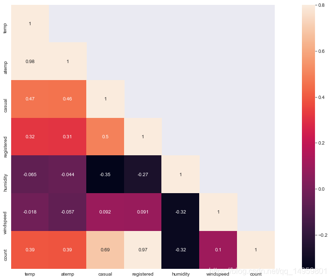
In [10]:
corrMatt = dailyData[["temp","atemp","casual","registered","humidity","windspeed","count"]].corr()
mask = np.array(corrMatt)
mask[np.tril_indices_from(mask)] = False
fig,ax= plt.subplots()
fig.set_size_inches(20,10)
sn.heatmap(corrMatt, mask=mask,vmax=.8, square=True,annot=True)
Out[10]:
<matplotlib.axes._subplots.AxesSubplot at 0xc355dd8>
In [11]:
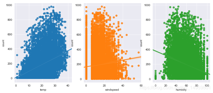
fig,(ax1,ax2,ax3) = plt.subplots(ncols=3)
fig.set_size_inches(12, 5)
sn.regplot(x="temp", y="count", data=dailyData,ax=ax1)
sn.regplot(x="windspeed", y="count", data=dailyData,ax=ax2)
sn.regplot(x="humidity", y="count", data=dailyData,ax=ax3)
Out[11]:
<matplotlib.axes._subplots.AxesSubplot at 0xa761cf8>
In [12]:
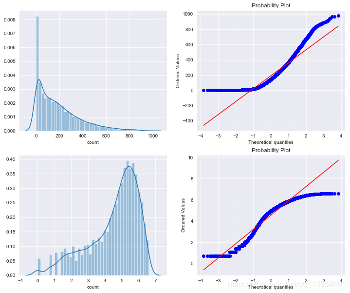
fig,axes = plt.subplots(ncols=2,nrows=2)
fig.set_size_inches(12, 10)
sn.distplot(dailyData["count"],ax=axes[0][0])
stats.probplot(dailyData["count"], dist='norm', fit=True, plot=axes[0][1])
sn.distplot(np.log(dailyDataWithoutOutliers["count"]),ax=axes[1][0])
stats.probplot(np.log1p(dailyDataWithoutOutliers["count"]), dist='norm', fit=True, plot=axes[1][1])
Out[12]:
((array([-3.82819677, -3.60401975, -3.48099008, ...,  3.48099008,
          3.60401975,  3.82819677]),
  array([0.69314718, 0.69314718, 0.69314718, ..., 6.5971457 , 6.59850903,
         6.5998705 ])),
 (1.3486990121229765, 4.562423868087808, 0.9581176780909608))
In [13]:
fig,(ax1,ax2,ax3,ax4)= plt.subplots(nrows=4)
fig.set_size_inches(12,20)
sortOrder = ["January","February","March","April","May","June","July","August","September","October","November","December"]
hueOrder = ["Sunday","Monday","Tuesday","Wednesday","Thursday","Friday","Saturday"]
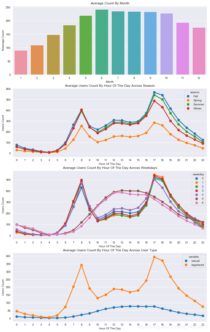
monthAggregated = pd.DataFrame(dailyData.groupby("month")["count"].mean()).reset_index()
sn.barplot(data=monthAggregated,x="month",y="count",ax=ax1)
ax1.set(xlabel='Month', ylabel='Avearage Count',title="Average Count By Month")
hourAggregated = pd.DataFrame(dailyData.groupby(["hour","season"],sort=True)["count"].mean()).reset_index()
sn.pointplot(x=hourAggregated["hour"], y=hourAggregated["count"],hue=hourAggregated["season"], data=hourAggregated, join=True,ax=ax2)
ax2.set(xlabel='Hour Of The Day', ylabel='Users Count',title="Average Users Count By Hour Of The Day Across Season",label='big')
hourAggregated = pd.DataFrame(dailyData.groupby(["hour","weekday"],sort=True)["count"].mean()).reset_index()
sn.pointplot(x=hourAggregated["hour"], y=hourAggregated["count"],hue=hourAggregated["weekday"], data=hourAggregated, join=True,ax=ax3)
ax3.set(xlabel='Hour Of The Day', ylabel='Users Count',title="Average Users Count By Hour Of The Day Across Weekdays",label='big')
hourTransformed = pd.melt(dailyData[["hour","casual","registered"]], id_vars=['hour'], value_vars=['casual', 'registered'])
hourAggregated = pd.DataFrame(hourTransformed.groupby(["hour","variable"],sort=True)["value"].mean()).reset_index()
sn.pointplot(x=hourAggregated["hour"], y=hourAggregated["value"],hue=hourAggregated["variable"],hue_order=["casual","registered"], data=hourAggregated, join=True,ax=ax4)
ax4.set(xlabel='Hour Of The Day', ylabel='Users Count',title="Average Users Count By Hour Of The Day Across User Type",label='big')
Out[13]:
[Text(0, 0.5, 'Users Count'),
 Text(0.5, 0, 'Hour Of The Day'),
 Text(0.5, 1.0, 'Average Users Count By Hour Of The Day Across User Type'),
 None]
In [14]:
dataTrain = pd.read_csv("C:/Users/_lc/BikeSharingDemand/train.csv")
dataTest = pd.read_csv("C:/Users/_lc/BikeSharingDemand/test.csv")
dataTest.head(2)
Out[14]:
| datetime | season | holiday | workingday | weather | temp | atemp | humidity | windspeed | |
|---|---|---|---|---|---|---|---|---|---|
| 0 | 2011-01-20 00:00:00 | 1 | 0 | 1 | 1 | 10.66 | 11.365 | 56 | 26.0027 |
| 1 | 2011-01-20 01:00:00 | 1 | 0 | 1 | 1 | 10.66 | 13.635 | 56 | 0.0000 |
In [35]:
data = dataTrain.append(dataTest)
data.reset_index(inplace=True)
data.drop('index',inplace=True,axis=1)
data.head()
Out[35]:
| atemp | casual | count | datetime | holiday | humidity | registered | season | temp | weather | windspeed | workingday | |
|---|---|---|---|---|---|---|---|---|---|---|---|---|
| 0 | 14.395 | 3.0 | 16.0 | 2011-01-01 00:00:00 | 0 | 81 | 13.0 | 1 | 9.84 | 1 | 0.0 | 0 |
| 1 | 13.635 | 8.0 | 40.0 | 2011-01-01 01:00:00 | 0 | 80 | 32.0 | 1 | 9.02 | 1 | 0.0 | 0 |
| 2 | 13.635 | 5.0 | 32.0 | 2011-01-01 02:00:00 | 0 | 80 | 27.0 | 1 | 9.02 | 1 | 0.0 | 0 |
| 3 | 14.395 | 3.0 | 13.0 | 2011-01-01 03:00:00 | 0 | 75 | 10.0 | 1 | 9.84 | 1 | 0.0 | 0 |
| 4 | 14.395 | 0.0 | 1.0 | 2011-01-01 04:00:00 | 0 | 75 | 1.0 | 1 | 9.84 | 1 | 0.0 | 0 |
In [36]:
data["datetime"] = pd.to_datetime(data.datetime)
data["year"] = data.datetime.map(lambda x : x.year)
data["month"] = data.datetime.apply(lambda x: x.month)
data["day"] = data.datetime.apply(lambda x : x.day)
data["hour"] = data.datetime.apply(lambda x : x.hour)
data['weekday'] = data.datetime.map(lambda x: x.weekday())
data.head()
Out[36]:
| atemp | casual | count | datetime | holiday | humidity | registered | season | temp | weather | windspeed | workingday | year | month | day | hour | weekday | |
|---|---|---|---|---|---|---|---|---|---|---|---|---|---|---|---|---|---|
| 0 | 14.395 | 3.0 | 16.0 | 2011-01-01 00:00:00 | 0 | 81 | 13.0 | 1 | 9.84 | 1 | 0.0 | 0 | 2011 | 1 | 1 | 0 | 5 |
| 1 | 13.635 | 8.0 | 40.0 | 2011-01-01 01:00:00 | 0 | 80 | 32.0 | 1 | 9.02 | 1 | 0.0 | 0 | 2011 | 1 | 1 | 1 | 5 |
| 2 | 13.635 | 5.0 | 32.0 | 2011-01-01 02:00:00 | 0 | 80 | 27.0 | 1 | 9.02 | 1 | 0.0 | 0 | 2011 | 1 | 1 | 2 | 5 |
| 3 | 14.395 | 3.0 | 13.0 | 2011-01-01 03:00:00 | 0 | 75 | 10.0 | 1 | 9.84 | 1 | 0.0 | 0 | 2011 | 1 | 1 | 3 | 5 |
| 4 | 14.395 | 0.0 | 1.0 | 2011-01-01 04:00:00 | 0 | 75 | 1.0 | 1 | 9.84 | 1 | 0.0 | 0 | 2011 | 1 | 1 | 4 | 5 |
In [37]:
# ---------预测风速为零的---------
from sklearn.ensemble import RandomForestRegressor
dataWind0 = data[data["windspeed"]==0]
dataWindNot0 = data[data["windspeed"]!=0]
rfModel_wind = RandomForestRegressor()
windColumns = ["season","weather","humidity","month","temp","year","atemp"]
rfModel_wind.fit(dataWindNot0[windColumns], dataWindNot0["windspeed"])

wind0Values = rfModel_wind.predict(X= dataWind0[windColumns])
dataWind0["windspeed"] = wind0Values
data = dataWindNot0.append(dataWind0)
data.reset_index(inplace=True)
data.drop('index',inplace=True,axis=1)
data.head()
C:\ProgramData\Anaconda3\lib\site-packages\sklearn\ensemble\forest.py:246: FutureWarning: The default value of n_estimators will change from 10 in version 0.20 to 100 in 0.22.
  "10 in version 0.20 to 100 in 0.22.", FutureWarning)
Out[37]:
| atemp | casual | count | datetime | holiday | humidity | registered | season | temp | weather | windspeed | workingday | year | month | day | hour | weekday | |
|---|---|---|---|---|---|---|---|---|---|---|---|---|---|---|---|---|---|
| 0 | 12.880 | 0.0 | 1.0 | 2011-01-01 05:00:00 | 0 | 75 | 1.0 | 1 | 9.84 | 2 | 6.0032 | 0 | 2011 | 1 | 1 | 5 | 5 |
| 1 | 19.695 | 12.0 | 36.0 | 2011-01-01 10:00:00 | 0 | 76 | 24.0 | 1 | 15.58 | 1 | 16.9979 | 0 | 2011 | 1 | 1 | 10 | 5 |
| 2 | 16.665 | 26.0 | 56.0 | 2011-01-01 11:00:00 | 0 | 81 | 30.0 | 1 | 14.76 | 1 | 19.0012 | 0 | 2011 | 1 | 1 | 11 | 5 |
| 3 | 21.210 | 29.0 | 84.0 | 2011-01-01 12:00:00 | 0 | 77 | 55.0 | 1 | 17.22 | 1 | 19.0012 | 0 | 2011 | 1 | 1 | 12 | 5 |
| 4 | 22.725 | 47.0 | 94.0 | 2011-01-01 13:00:00 | 0 | 72 | 47.0 | 1 | 18.86 | 2 | 19.9995 | 0 | 2011 | 1 | 1 | 13 | 5 |
In [39]:
categoricalFeatureNames = ["season","holiday","workingday","weather","weekday","month","year","hour"]
numericalFeatureNames = ["temp","humidity","windspeed","atemp"]
dropFeatures = ['casual',"count","datetime","day","registered"]
for var in categoricalFeatureNames:
    data[var] = data[var].astype("category")
In [40]:
dataTrain = data[pd.notnull(data['count'])].sort_values(by=["datetime"])
dataTest = data[~pd.notnull(data['count'])].sort_values(by=["datetime"])
datetimecol = dataTest["datetime"]
yLabels = dataTrain["count"]
yLablesRegistered = dataTrain["registered"]
yLablesCasual = dataTrain["casual"]

dataTrain  = dataTrain.drop(dropFeatures,axis=1)
dataTest  = dataTest.drop(dropFeatures,axis=1)
In [47]:
# 对数均方误差
def rmsle(y, y_,convertExp=True):
    if convertExp:
        y = np.exp(y),
        y_ = np.exp(y_)
    log1 = np.nan_to_num(np.array([np.log(v + 1) for v in y]))
    log2 = np.nan_to_num(np.array([np.log(v + 1) for v in y_]))
    calc = (log1 - log2) ** 2
    return np.sqrt(np.mean(calc))
In [48]:
from sklearn.linear_model import LinearRegression,Ridge,Lasso
from sklearn.model_selection import GridSearchCV
from sklearn import metrics
import warnings
pd.options.mode.chained_assignment = None
warnings.filterwarnings("ignore", category=DeprecationWarning)

lModel = LinearRegression()

yLabelsLog = np.log1p(yLabels)
lModel.fit(X = dataTrain,y = yLabelsLog)

preds = lModel.predict(X= dataTrain)
print ("RMSLE Value For Linear Regression: ",rmsle(np.exp(yLabelsLog),np.exp(preds),False))
RMSLE Value For Linear Regression: 0.9779688131592883
In [53]:
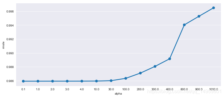
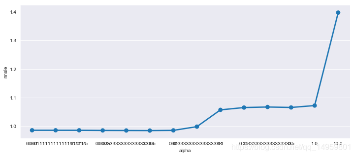
ridge_m_ = Ridge()
ridge_params_ = { 'max_iter':[3000],'alpha':[0.1, 1, 2, 3, 4, 10, 30,100,200,300,400,800,900,1000]}
rmsle_scorer = metrics.make_scorer(rmsle, greater_is_better=False)
grid_ridge_m = GridSearchCV( ridge_m_,
                          ridge_params_,
                          scoring = rmsle_scorer,
                          cv=5)
yLabelsLog = np.log1p(yLabels)
grid_ridge_m.fit( dataTrain, yLabelsLog )
preds = grid_ridge_m.predict(X= dataTrain)
print (grid_ridge_m.best_params_)
print ("RMSLE Value For Ridge Regression: ",rmsle(np.exp(yLabelsLog),np.exp(preds),False))

fig,ax= plt.subplots()
fig.set_size_inches(12,5)
df = pd.DataFrame(grid_ridge_m.cv_results_)
df["alpha"] = df["params"].apply(lambda x:x["alpha"])
df["rmsle"] = df["mean_test_score"].apply(lambda x:-x)
sn.pointplot(data=df,x="alpha",y="rmsle",ax=ax)
{'alpha': 0.1, 'max_iter': 3000}
RMSLE Value For Ridge Regression:  0.9779687981095982
Out[53]:
<matplotlib.axes._subplots.AxesSubplot at 0x12c49cc0>
In [55]:
lasso_m_ = Lasso()

alpha  = 1/np.array([0.1, 1, 2, 3, 4, 10, 30,100,200,300,400,800,900,1000])
lasso_params_ = { 'max_iter':[3000],'alpha':alpha}

grid_lasso_m = GridSearchCV( lasso_m_,lasso_params_,scoring = rmsle_scorer,cv=5)
yLabelsLog = np.log1p(yLabels)
grid_lasso_m.fit( dataTrain, yLabelsLog )
preds = grid_lasso_m.predict(X= dataTrain)
print (grid_lasso_m.best_params_)
print ("RMSLE Value For Lasso Regression: ",rmsle(np.exp(yLabelsLog),np.exp(preds),False))

fig,ax= plt.subplots()
fig.set_size_inches(12,5)
df = pd.DataFrame(grid_lasso_m.cv_results_)
df["alpha"] = df["params"].apply(lambda x:x["alpha"])
df["rmsle"] = df["mean_test_score"].apply(lambda x:-x)
sn.pointplot(data=df,x="alpha",y="rmsle",ax=ax)
{'alpha': 0.005, 'max_iter': 3000}
RMSLE Value For Lasso Regression:  0.9781068303163186
Out[55]:
<matplotlib.axes._subplots.AxesSubplot at 0x12dbd080>
In [56]:
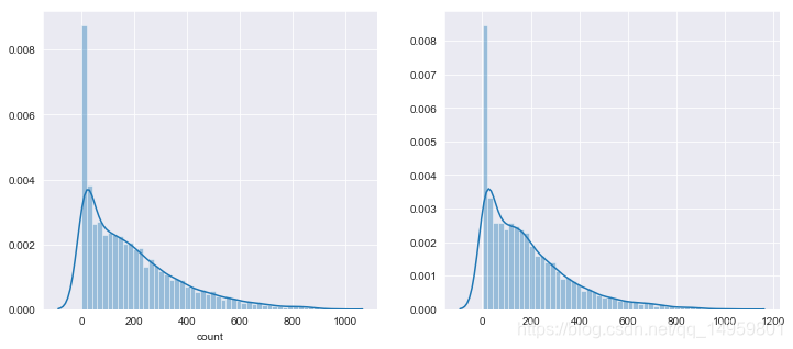
from sklearn.ensemble import GradientBoostingRegressor
gbm = GradientBoostingRegressor(n_estimators=4000,alpha=0.01); ### Test 0.41
yLabelsLog = np.log1p(yLabels)
gbm.fit(dataTrain,yLabelsLog)
preds = gbm.predict(X= dataTrain)
print ("RMSLE Value For Gradient Boost: ",rmsle(np.exp(yLabelsLog),np.exp(preds),False))

predsTest = gbm.predict(X= dataTest)
fig,(ax1,ax2)= plt.subplots(ncols=2)
fig.set_size_inches(12,5)
sn.distplot(yLabels,ax=ax1,bins=50)
sn.distplot(np.exp(predsTest),ax=ax2,bins=50)
RMSLE Value For Gradient Boost: 0.1896091619650034
Out[56]:
<matplotlib.axes._subplots.AxesSubplot at 0x14104278>


 3864
3864

 被折叠的 条评论
为什么被折叠?
被折叠的 条评论
为什么被折叠?
 到【灌水乐园】发言


