【机器学习chp7代码示例】SVM分类和回归、线性核和径向基核

目录

一、分类—SVC

二、回归—SVR

---

一、分类—SVC

import numpy as np
import matplotlib.pyplot as plt
from matplotlib.colors import ListedColormap
from sklearn.model_selection import train_test_split
from sklearn.preprocessing import StandardScaler
from sklearn.datasets import make_moons, make_circles, make_classification
from sklearn.svm import SVC

names = ["Linear SVM", "RBF SVM"]


classifiers = [
    SVC(kernel="linear", C=0.025),
    SVC(gamma=2, C=1)]

X, y = make_classification(n_features=2, n_redundant=0, n_informative=2,
                           random_state=1, n_clusters_per_class=1)


rng = np.random.RandomState(2)
X += 2 * rng.uniform(size=X.shape)
linearly_separable = (X, y)

datasets = [make_moons(noise=0.3, random_state=0),
            make_circles(noise=0.2, factor=0.5, random_state=1),
            linearly_separable
            ]

figure = plt.figure(figsize=(9, 9))
i = 1

# iterate over datasets
for ds_cnt, ds in enumerate(datasets):
    # preprocess dataset, split into training and test part
    X, y = ds
    X = StandardScaler().fit_transform(X)
    X_train, X_test, y_train, y_test = \
        train_test_split(X, y, test_size=.4, random_state=42)

    x_min, x_max = X[:, 0].min() - .5, X[:, 0].max() + .5
    y_min, y_max = X[:, 1].min() - .5, X[:, 1].max() + .5
    xx, yy = np.meshgrid(np.arange(x_min, x_max, h),
                         np.arange(y_min, y_max, h))

    # just plot the dataset first
    cm = plt.cm.RdBu
    cm_bright = ListedColormap(['#FF0000', '#0000FF'])
    ax = plt.subplot(len(datasets), len(classifiers) + 1, i)
    if ds_cnt == 0:
        ax.set_title("Input data")
    # Plot the training points
    ax.scatter(X_train[:, 0], X_train[:, 1], c=y_train, cmap=cm_bright,
               edgecolors='k')
    # Plot the testing points
    ax.scatter(X_test[:, 0], X_test[:, 1], c=y_test, cmap=cm_bright, alpha=0.6,
               edgecolors='k')
    ax.set_xlim(xx.min(), xx.max())
    ax.set_ylim(yy.min(), yy.max())
    ax.set_xticks(())
    ax.set_yticks(())
    i += 1

    # iterate over classifiers
    for name, clf in zip(names, classifiers):
        ax = plt.subplot(len(datasets), len(classifiers) + 1, i)
        clf.fit(X_train, y_train)
        score = clf.score(X_test, y_test)

        # Plot the decision boundary. For that, we will assign a color to each
        # point in the mesh [x_min, x_max]x[y_min, y_max].
        if hasattr(clf, "decision_function"):
            Z = clf.decision_function(np.c_[xx.ravel(), yy.ravel()])
        else:
            Z = clf.predict_proba(np.c_[xx.ravel(), yy.ravel()])[:, 1]

        # Put the result into a color plot
        Z = Z.reshape(xx.shape)
        ax.contourf(xx, yy, Z, cmap=cm, alpha=.8)

        # Plot the training points
        ax.scatter(X_train[:, 0], X_train[:, 1], c=y_train, cmap=cm_bright,
                   edgecolors='k')
        # Plot the testing points
        ax.scatter(X_test[:, 0], X_test[:, 1], c=y_test, cmap=cm_bright,
                   edgecolors='k', alpha=0.6)

        ax.set_xlim(xx.min(), xx.max())
        ax.set_ylim(yy.min(), yy.max())
        ax.set_xticks(())
        ax.set_yticks(())
        if ds_cnt == 0:
            ax.set_title(name)
        ax.text(xx.max() - .3, yy.min() + .3, ('%.2f' % score).lstrip('0'),
                size=15, horizontalalignment='right')
        i += 1

plt.tight_layout()
plt.show()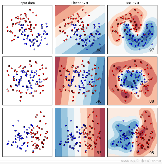

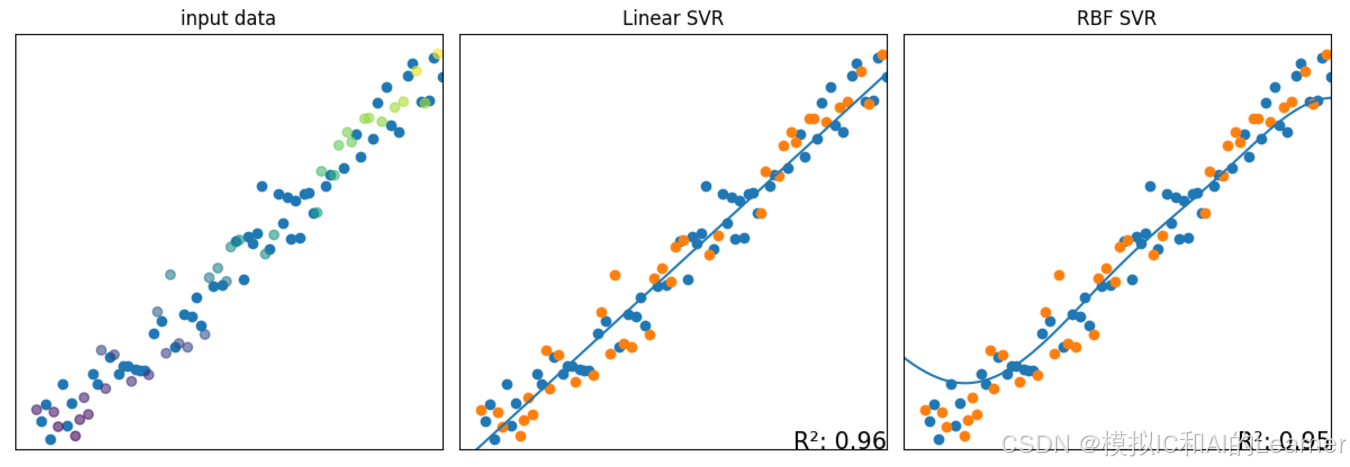
二、回归—SVR

import numpy as np
import matplotlib.pyplot as plt
from matplotlib.colors import ListedColormap
from sklearn.model_selection import train_test_split
from sklearn.preprocessing import StandardScaler
from sklearn.datasets import make_regression
from sklearn.svm import SVR

# 定义SVR回归器名称和模型
names = ["Linear SVR", "RBF SVR"]
regressors = [
    SVR(kernel="linear", C=1.0, epsilon=0.1),
    SVR(kernel="rbf", C=1.0, gamma="scale", epsilon=0.1)
]

# 生成数据集
# 数据集1：线性回归数据集: y = 2x + 1
X_lin = np.linspace(0, 10, 100)
y_lin = 2 * X_lin + 1 + np.random.normal(0, 1, size=100)
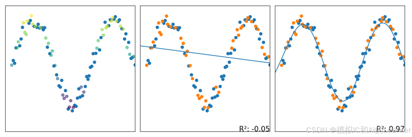
# 数据集2：非线性回归数据集（正弦关系）: y = sin(x)
X_sin = np.linspace(0, 10, 100)
y_sin = np.sin(X_sin) + np.random.normal(0, 0.1, size=100)
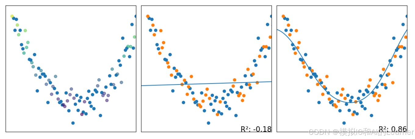
# 数据集3：二次曲线回归数据集：y = 0.2x^2 - 2x + 5
X_quad = np.linspace(0, 10, 100)
y_quad = 0.2 * X_quad**2 - 2 * X_quad + 5 + np.random.normal(0, 0.5, size=100)

datasets = [(X_lin, y_lin), (X_sin, y_sin), (X_quad, y_quad)]

figure = plt.figure(figsize=(12, 12))
i = 1
h = 1  # 网格步长

# 遍历每个数据集
for ds_cnt, ds in enumerate(datasets):
    X, y = ds
    # 划分训练集和测试集
    X_train, X_test, y_train, y_test = train_test_split(X, y, test_size=0.4, random_state=42)
    
    # 定义网格边界
    x_min, x_max = X.min()-0.5 , X.max()+0.5
    y_min, y_max = y.min()-0.5 , y.max()+0.5
    xx, yy = np.meshgrid(np.arange(x_min, x_max, h),
                         np.arange(y_min, y_max, h))
    
    # 第一个子图：绘制原始数据（训练集和测试集）
    ax = plt.subplot(len(datasets), len(regressors) + 1, i)
    if ds_cnt == 0:
        ax.set_title("input data")
    sc = ax.scatter(X_train, y_train)
    ax.scatter(X_test, y_test, c=y_test,  alpha=0.6)
    ax.set_xlim(xx.min(), xx.max())
    ax.set_ylim(yy.min(), yy.max())
    ax.set_xticks(())
    ax.set_yticks(())

    i += 1
    
    # 遍历每个SVR模型
    for name, reg in zip(names, regressors):
        ax = plt.subplot(len(datasets), len(regressors) + 1, i)
        X_train = np.array(X_train).reshape(-1, 1)
        reg.fit(X_train,y_train)
        X_test = np.array(X_test).reshape(-1, 1)
        
        score = reg.score(X_test, y_test)  # R²得分
        
        
        # 绘制训练和测试数据点
        sc_train = ax.scatter(X_train, y_train)
        ax.scatter(X_test, y_test)
        ax.set_xlim(xx.min(), xx.max())
        ax.set_ylim(yy.min(), yy.max())
        ax.set_xticks(())
        ax.set_yticks(())
        if ds_cnt == 0:
            ax.set_title(name)
        ax.text(xx.max(), yy.min(), f'R²: {score:.2f}', size=15,
                horizontalalignment='right')
        #绘制回归线
        X_pic = np.linspace(xx.min(), xx.max(), int(10*(xx.max()-xx.min())))
        X_pic = np.array(X_pic).reshape(-1, 1)
        y_pic = reg.predict(X_pic)
        ax.plot(X_pic, y_pic)


        i += 1

plt.tight_layout()
plt.show()