


目录
3、 Bagging 的一种变体:随机森林(包括极度随机森林)——分类
4、Bagging 的一种变体:随机森林(包括极度随机森林)——回归
一、Bagging
1、BaggingClassifier——分类
#Bagging——SVM、决策树——分类
import numpy as np
import matplotlib.pyplot as plt
from matplotlib.colors import ListedColormap
from sklearn.model_selection import train_test_split
from sklearn.preprocessing import StandardScaler
from sklearn.datasets import make_moons, make_circles, make_classification

from sklearn.svm import SVC
from sklearn.ensemble import BaggingClassifier


names = ["Bagging SVM", "Bagging Tree"]


classifiers = [
    BaggingClassifier(estimator=SVC(), n_estimators=10, random_state=0),
    BaggingClassifier(estimator=None, n_estimators=10, random_state=0)] #估计器默认是决策树

X, y = make_classification(n_features=2, n_redundant=0, n_informative=2,
                           random_state=1, n_clusters_per_class=1)


rng = np.random.RandomState(2)
X += 2 * rng.uniform(size=X.shape)
linearly_separable = (X, y)

datasets = [make_moons(noise=0.3, random_state=0),
            make_circles(noise=0.2, factor=0.5, random_state=1),
            linearly_separable
            ]

figure = plt.figure(figsize=(3*len(names)+3, 3*len(datasets)))
i = 1

# iterate over datasets
for ds_cnt, ds in enumerate(datasets):
    # preprocess dataset, split into training and test part
    X, y = ds
    X = StandardScaler().fit_transform(X)
    X_train, X_test, y_train, y_test = \
        train_test_split(X, y, test_size=.4, random_state=42)

    x_min, x_max = X[:, 0].min() - 1, X[:, 0].max() + 2
    y_min, y_max = X[:, 1].min() - 1, X[:, 1].max() + 1
    xx, yy = np.meshgrid(np.arange(x_min, x_max),
                         np.arange(y_min, y_max))

    # just plot the dataset first
    cm = plt.cm.RdBu
    cm_bright = ListedColormap(['#FF0000', '#0000FF'])
    ax = plt.subplot(len(datasets), len(classifiers) + 1, i)
    if ds_cnt == 0:
        ax.set_title("Input data")
    # Plot the training points
    ax.scatter(X_train[:, 0], X_train[:, 1], c=y_train, cmap=cm_bright,
               edgecolors='k')
    # Plot the testing points
    ax.scatter(X_test[:, 0], X_test[:, 1], c=y_test, cmap=cm_bright, alpha=0.6,
               edgecolors='k')
    ax.set_xlim(xx.min(), xx.max())
    ax.set_ylim(yy.min(), yy.max())
    ax.set_xticks(())
    ax.set_yticks(())
    i += 1

    # iterate over classifiers
    for name, clf in zip(names, classifiers):
        ax = plt.subplot(len(datasets), len(classifiers) + 1, i)
        clf.fit(X_train, y_train)
        score = clf.score(X_test, y_test)

        # Plot the decision boundary. For that, we will assign a color to each
        # point in the mesh [x_min, x_max]x[y_min, y_max].
        if hasattr(clf, "decision_function"):
            Z = clf.decision_function(np.c_[xx.ravel(), yy.ravel()])
        else:
            Z = clf.predict_proba(np.c_[xx.ravel(), yy.ravel()])[:, 1]

        # Put the result into a color plot
        Z = Z.reshape(xx.shape)
        ax.contourf(xx, yy, Z, cmap=cm, alpha=.8)

        # Plot the training points
        ax.scatter(X_train[:, 0], X_train[:, 1], c=y_train, cmap=cm_bright,
                   edgecolors='k')
        # Plot the testing points
        ax.scatter(X_test[:, 0], X_test[:, 1], c=y_test, cmap=cm_bright,
                   edgecolors='k', alpha=0.6)

        ax.set_xlim(xx.min(), xx.max())
        ax.set_ylim(yy.min(), yy.max())
        ax.set_xticks(())
        ax.set_yticks(())
        if ds_cnt == 0:
            ax.set_title(name)
        ax.text(xx.max() - .3, yy.min() + .3, ('%.2f' % score).lstrip('0'),
                size=15, horizontalalignment='right')
        i += 1

plt.tight_layout()
plt.show()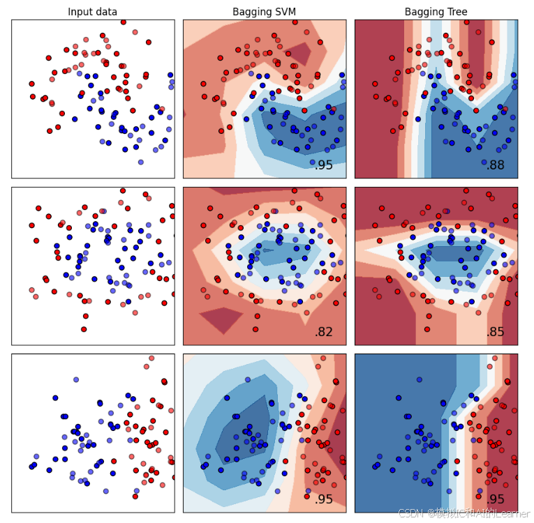
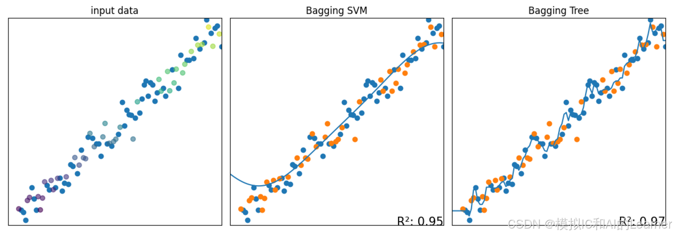
2、BaggingRegressor——回归
#Bagging——SVM、决策树——回归
import numpy as np
import matplotlib.pyplot as plt
from matplotlib.colors import ListedColormap
from sklearn.model_selection import train_test_split
from sklearn.preprocessing import StandardScaler
from sklearn.datasets import make_regression
from sklearn.svm import SVR
from sklearn.ensemble import BaggingRegressor
# 定义回归器名称和模型
names = ["Bagging SVM", "Bagging Tree"]
regressors = [
BaggingRegressor(estimator=SVR(), n_estimators=10, random_state=0),
BaggingRegressor(estimator=None, n_estimators=10, random_state=0)
]
# 生成数据集
# 数据集1:线性回归数据集: y = 2x + 1
X_lin = np.linspace(0, 10, 100)
y_lin = 2 * X_lin + 1 + np.random.normal(0, 1, size=100)
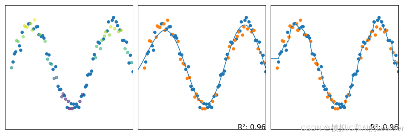
# 数据集2:非线性回归数据集(正弦关系): y = sin(x)
X_sin = np.linspace(0, 10, 100)
y_sin = np.sin(X_sin) + np.random.normal(0, 0.1, size=100)
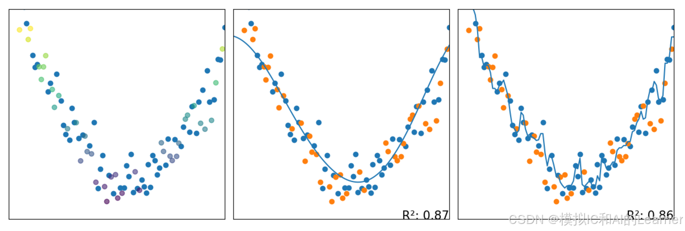
# 数据集3:二次曲线回归数据集:y = 0.2x^2 - 2x + 5
X_quad = np.linspace(0, 10, 100)
y_quad = 0.2 * X_quad**2 - 2 * X_quad + 5 + np.random.normal(0, 0.5, size=100)
datasets = [(X_lin, y_lin), (X_sin, y_sin), (X_quad, y_quad)]
figure = plt.figure(figsize=(3*len(names)+3, 3*len(datasets)))
i = 1
h = 1 # 网格步长
# 遍历每个数据集
for ds_cnt, ds in enumerate(datasets):
X, y = ds
# 划分训练集和测试集
X_train, X_test, y_train, y_test = train_test_split(X, y, test_size=0.4, random_state=42)
# 定义网格边界
x_min, x_max = X.min()-1 , X.max()+2
y_min, y_max = y.min()-1 , y.max()+2
xx, yy = np.meshgrid(np.arange(x_min, x_max, h),
np.arange(y_min, y_max, h))
# 第一个子图:绘制原始数据(训练集和测试集)
ax = plt.subplot(len(datasets), len(regressors) + 1, i)
if ds_cnt == 0:
ax.set_title("input data")
sc = ax.scatter(X_train, y_train)
ax.scatter(X_test, y_test, c=y_test, alpha=0.6)
ax.set_xlim(xx.min(), xx.max())
ax.set_ylim(yy.min(), yy.max())
ax.set_xticks(())
ax.set_yticks(())
i += 1
# 遍历每个SVR模型
for name, reg in zip(names, regressors):
ax = plt.subplot(len(datasets), len(regressors) + 1, i)
X_train = np.array(X_train).reshape(-1, 1)
reg.fit(X_train,y_train)
X_test = np.array(X_test).reshape(-1, 1)
score = reg.score(X_test, y_test) # R²得分
# 绘制训练和测试数据点
sc_train = ax.scatter(X_train, y_train)
ax.scatter(X_test, y_test)
ax.set_xlim(xx.min(), xx.max())
ax.set_ylim(yy.min(), yy.max())
ax.set_xticks(())
ax.set_yticks(())
if ds_cnt == 0:
ax.set_title(name)
ax.text(xx.max(), yy.min(), f'R²: {score:.2f}', size=15,
horizontalalignment='right')
#绘制回归线
X_pic = np.linspace(xx.min(), xx.max(), int(10*(xx.max()-xx.min())))
X_pic = np.array(X_pic).reshape(-1, 1)
y_pic = reg.predict(X_pic)
ax.plot(X_pic, y_pic)
i += 1
plt.tight_layout()
plt.show()
3、 Bagging 的一种变体:随机森林(包括极度随机森林)——分类
#Bagging变体——随机森林(包括极度随机森林)——分类

import numpy as np
import matplotlib.pyplot as plt
from matplotlib.colors import ListedColormap
from sklearn.model_selection import train_test_split
from sklearn.preprocessing import StandardScaler
from sklearn.datasets import make_moons, make_circles, make_classification

from sklearn.svm import SVC
from sklearn.ensemble import RandomForestClassifier
from sklearn.ensemble import ExtraTreesClassifier


names = ["RandomForest","ExtraTrees"]


classifiers = [
    RandomForestClassifier(max_depth=5, n_estimators=100, max_features=1),
    ExtraTreesClassifier(max_depth=5, n_estimators=100, random_state=0)
    ]

X, y = make_classification(n_features=2, n_redundant=0, n_informative=2,
                           random_state=1, n_clusters_per_class=1)


rng = np.random.RandomState(2)
X += 2 * rng.uniform(size=X.shape)
linearly_separable = (X, y)

datasets = [make_moons(noise=0.3, random_state=0),
            make_circles(noise=0.2, factor=0.5, random_state=1),
            linearly_separable
            ]

figure = plt.figure(figsize=(3*len(names)+3, 3*len(datasets)))
i = 1

# iterate over datasets
for ds_cnt, ds in enumerate(datasets):
    # preprocess dataset, split into training and test part
    X, y = ds
    X = StandardScaler().fit_transform(X)
    X_train, X_test, y_train, y_test = \
        train_test_split(X, y, test_size=.4, random_state=42)

    x_min, x_max = X[:, 0].min() - 1, X[:, 0].max() + 2
    y_min, y_max = X[:, 1].min() - 1, X[:, 1].max() + 1
    xx, yy = np.meshgrid(np.arange(x_min, x_max),
                         np.arange(y_min, y_max))

    # just plot the dataset first
    cm = plt.cm.RdBu
    cm_bright = ListedColormap(['#FF0000', '#0000FF'])
    ax = plt.subplot(len(datasets), len(classifiers) + 1, i)
    if ds_cnt == 0:
        ax.set_title("Input data")
    # Plot the training points
    ax.scatter(X_train[:, 0], X_train[:, 1], c=y_train, cmap=cm_bright,
               edgecolors='k')
    # Plot the testing points
    ax.scatter(X_test[:, 0], X_test[:, 1], c=y_test, cmap=cm_bright, alpha=0.6,
               edgecolors='k')
    ax.set_xlim(xx.min(), xx.max())
    ax.set_ylim(yy.min(), yy.max())
    ax.set_xticks(())
    ax.set_yticks(())
    i += 1

    # iterate over classifiers
    for name, clf in zip(names, classifiers):
        ax = plt.subplot(len(datasets), len(classifiers) + 1, i)
        clf.fit(X_train, y_train)
        score = clf.score(X_test, y_test)

        # Plot the decision boundary. For that, we will assign a color to each
        # point in the mesh [x_min, x_max]x[y_min, y_max].
        if hasattr(clf, "decision_function"):
            Z = clf.decision_function(np.c_[xx.ravel(), yy.ravel()])
        else:
            Z = clf.predict_proba(np.c_[xx.ravel(), yy.ravel()])[:, 1]

        # Put the result into a color plot
        Z = Z.reshape(xx.shape)
        ax.contourf(xx, yy, Z, cmap=cm, alpha=.8)

        # Plot the training points
        ax.scatter(X_train[:, 0], X_train[:, 1], c=y_train, cmap=cm_bright,
                   edgecolors='k')
        # Plot the testing points
        ax.scatter(X_test[:, 0], X_test[:, 1], c=y_test, cmap=cm_bright,
                   edgecolors='k', alpha=0.6)

        ax.set_xlim(xx.min(), xx.max())
        ax.set_ylim(yy.min(), yy.max())
        ax.set_xticks(())
        ax.set_yticks(())
        if ds_cnt == 0:
            ax.set_title(name)
        ax.text(xx.max() - .3, yy.min() + .3, ('%.2f' % score).lstrip('0'),
                size=15, horizontalalignment='right')
        i += 1

plt.tight_layout()
plt.show()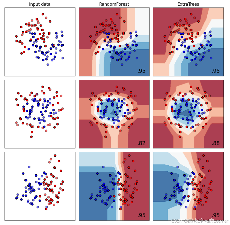
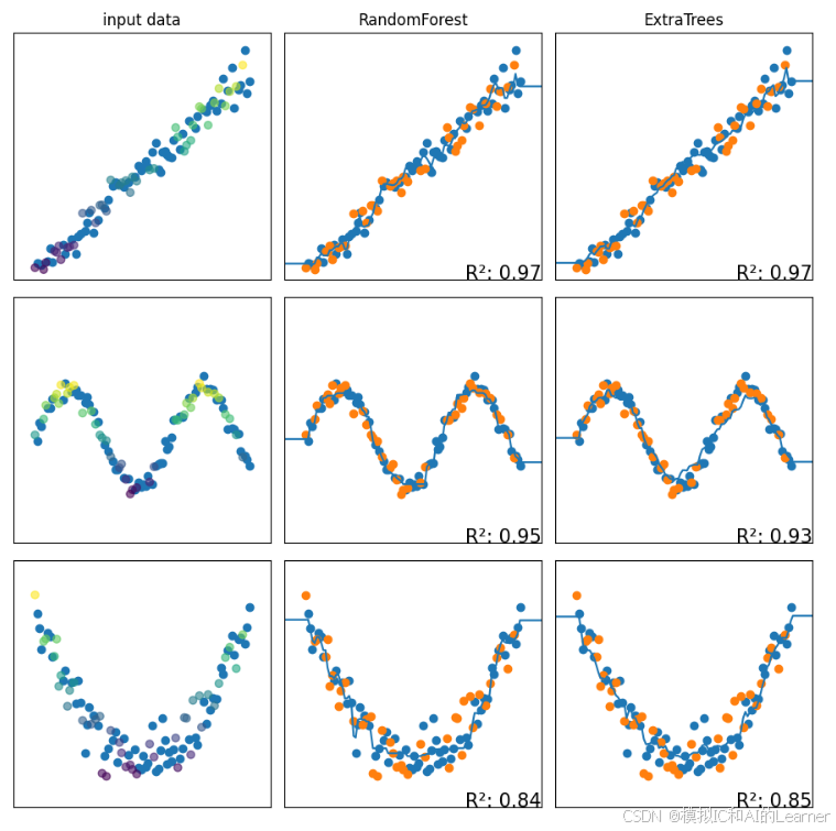
4、Bagging 的一种变体:随机森林(包括极度随机森林)——回归
#Bagging变体——随机森林(包括嫉妒随机森林)——回归

import numpy as np
import matplotlib.pyplot as plt
from matplotlib.colors import ListedColormap
from sklearn.model_selection import train_test_split
from sklearn.preprocessing import StandardScaler
from sklearn.datasets import make_regression

from sklearn.svm import SVR
from sklearn.ensemble import RandomForestRegressor
from sklearn.ensemble import ExtraTreesRegressor

# 定义回归器名称和模型
names = ["RandomForest","ExtraTrees"]
regressors = [
    RandomForestRegressor(max_depth=5, n_estimators=10, max_features=1),
    ExtraTreesRegressor(max_depth=5, n_estimators=10, random_state=0)
]

# 生成数据集
# 数据集1:线性回归数据集: y = 2x + 1
X_lin = np.linspace(0, 10, 100)
y_lin = 2 * X_lin + 1 + np.random.normal(0, 1, size=100)
# 数据集2:非线性回归数据集(正弦关系): y = sin(x)
X_sin = np.linspace(0, 10, 100)
y_sin = np.sin(X_sin) + np.random.normal(0, 0.1, size=100)
# 数据集3:二次曲线回归数据集:y = 0.2x^2 - 2x + 5
X_quad = np.linspace(0, 10, 100)
y_quad = 0.2 * X_quad**2 - 2 * X_quad + 5 + np.random.normal(0, 0.5, size=100)

datasets = [(X_lin, y_lin), (X_sin, y_sin), (X_quad, y_quad)]

figure = plt.figure(figsize=(3*len(names)+3, 3*len(datasets)))
i = 1
h = 1  # 网格步长

# 遍历每个数据集
for ds_cnt, ds in enumerate(datasets):
    X, y = ds
    # 划分训练集和测试集
    X_train, X_test, y_train, y_test = train_test_split(X, y, test_size=0.4, random_state=42)

    # 定义网格边界
    x_min, x_max = X.min()-1 , X.max()+2
    y_min, y_max = y.min()-1 , y.max()+2
    xx, yy = np.meshgrid(np.arange(x_min, x_max, h),
                         np.arange(y_min, y_max, h))

    # 第一个子图:绘制原始数据(训练集和测试集)
    ax = plt.subplot(len(datasets), len(regressors) + 1, i)
    if ds_cnt == 0:
        ax.set_title("input data")
    sc = ax.scatter(X_train, y_train)
    ax.scatter(X_test, y_test, c=y_test,  alpha=0.6)
    ax.set_xlim(xx.min(), xx.max())
    ax.set_ylim(yy.min(), yy.max())
    ax.set_xticks(())
    ax.set_yticks(())

    i += 1

    # 遍历每个SVR模型
    for name, reg in zip(names, regressors):
        ax = plt.subplot(len(datasets), len(regressors) + 1, i)
        X_train = np.array(X_train).reshape(-1, 1)
        reg.fit(X_train,y_train)
        X_test = np.array(X_test).reshape(-1, 1)

        score = reg.score(X_test, y_test)  # R²得分


        # 绘制训练和测试数据点
        sc_train = ax.scatter(X_train, y_train)
        ax.scatter(X_test, y_test)
        ax.set_xlim(xx.min(), xx.max())
        ax.set_ylim(yy.min(), yy.max())
        ax.set_xticks(())
        ax.set_yticks(())
        if ds_cnt == 0:
            ax.set_title(name)
        ax.text(xx.max(), yy.min(), f'R²: {score:.2f}', size=15,
                horizontalalignment='right')
        #绘制回归线
        X_pic = np.linspace(xx.min(), xx.max(), int(10*(xx.max()-xx.min())))
        X_pic = np.array(X_pic).reshape(-1, 1)
        y_pic = reg.predict(X_pic)
        ax.plot(X_pic, y_pic)


        i += 1

plt.tight_layout()
plt.show()
二、Boosting提升法
1、AdaBoost——分类
#提升法——AdaBoost——分类


import numpy as np
import matplotlib.pyplot as plt
from matplotlib.colors import ListedColormap
from sklearn.model_selection import train_test_split
from sklearn.preprocessing import StandardScaler
from sklearn.datasets import make_moons, make_circles, make_classification

from sklearn.svm import SVC
from sklearn.ensemble import AdaBoostClassifier


names = ["AdaBoost"]


classifiers = [
    AdaBoostClassifier()
    ]

X, y = make_classification(n_features=2, n_redundant=0, n_informative=2,
                           random_state=1, n_clusters_per_class=1)


rng = np.random.RandomState(2)
X += 2 * rng.uniform(size=X.shape)
linearly_separable = (X, y)

datasets = [make_moons(noise=0.3, random_state=0),
            make_circles(noise=0.2, factor=0.5, random_state=1),
            linearly_separable
            ]

figure = plt.figure(figsize=(3*len(names)+3, 3*len(datasets)))
i = 1

# iterate over datasets
for ds_cnt, ds in enumerate(datasets):
    # preprocess dataset, split into training and test part
    X, y = ds
    X = StandardScaler().fit_transform(X)
    X_train, X_test, y_train, y_test = \
        train_test_split(X, y, test_size=.4, random_state=42)

    x_min, x_max = X[:, 0].min() - 1, X[:, 0].max() + 2
    y_min, y_max = X[:, 1].min() - 1, X[:, 1].max() + 1
    xx, yy = np.meshgrid(np.arange(x_min, x_max),
                         np.arange(y_min, y_max))

    # just plot the dataset first
    cm = plt.cm.RdBu
    cm_bright = ListedColormap(['#FF0000', '#0000FF'])
    ax = plt.subplot(len(datasets), len(classifiers) + 1, i)
    if ds_cnt == 0:
        ax.set_title("Input data")
    # Plot the training points
    ax.scatter(X_train[:, 0], X_train[:, 1], c=y_train, cmap=cm_bright,
               edgecolors='k')
    # Plot the testing points
    ax.scatter(X_test[:, 0], X_test[:, 1], c=y_test, cmap=cm_bright, alpha=0.6,
               edgecolors='k')
    ax.set_xlim(xx.min(), xx.max())
    ax.set_ylim(yy.min(), yy.max())
    ax.set_xticks(())
    ax.set_yticks(())
    i += 1

    # iterate over classifiers
    for name, clf in zip(names, classifiers):
        ax = plt.subplot(len(datasets), len(classifiers) + 1, i)
        clf.fit(X_train, y_train)
        score = clf.score(X_test, y_test)

        # Plot the decision boundary. For that, we will assign a color to each
        # point in the mesh [x_min, x_max]x[y_min, y_max].
        if hasattr(clf, "decision_function"):
            Z = clf.decision_function(np.c_[xx.ravel(), yy.ravel()])
        else:
            Z = clf.predict_proba(np.c_[xx.ravel(), yy.ravel()])[:, 1]

        # Put the result into a color plot
        Z = Z.reshape(xx.shape)
        ax.contourf(xx, yy, Z, cmap=cm, alpha=.8)

        # Plot the training points
        ax.scatter(X_train[:, 0], X_train[:, 1], c=y_train, cmap=cm_bright,
                   edgecolors='k')
        # Plot the testing points
        ax.scatter(X_test[:, 0], X_test[:, 1], c=y_test, cmap=cm_bright,
                   edgecolors='k', alpha=0.6)

        ax.set_xlim(xx.min(), xx.max())
        ax.set_ylim(yy.min(), yy.max())
        ax.set_xticks(())
        ax.set_yticks(())
        if ds_cnt == 0:
            ax.set_title(name)
        ax.text(xx.max() - .3, yy.min() + .3, ('%.2f' % score).lstrip('0'),
                size=15, horizontalalignment='right')
        i += 1

plt.tight_layout()
plt.show()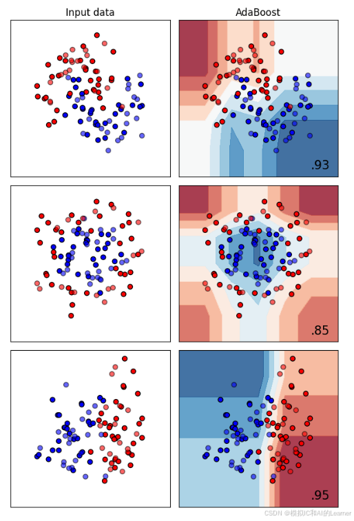
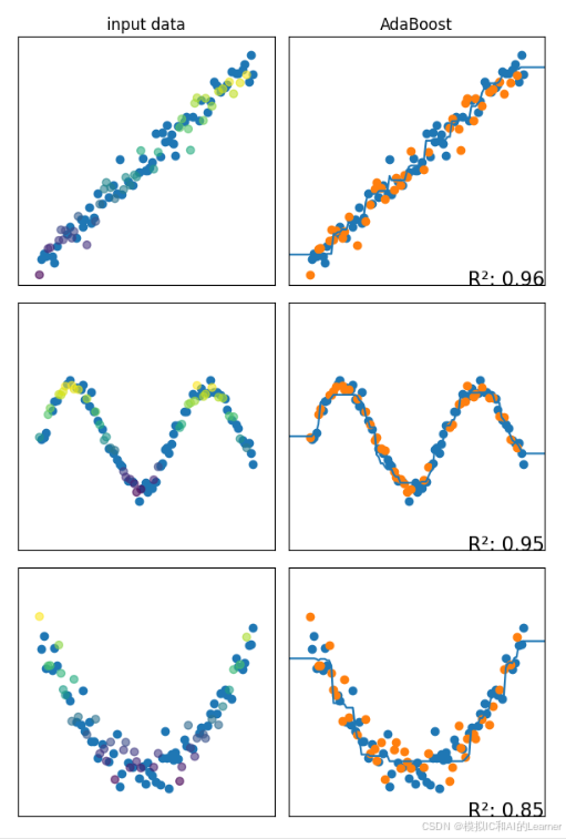
2、AdaBoost——回归
#提升法——AdaBoost——回归


import numpy as np
import matplotlib.pyplot as plt
from matplotlib.colors import ListedColormap
from sklearn.model_selection import train_test_split
from sklearn.preprocessing import StandardScaler
from sklearn.datasets import make_regression


from sklearn.ensemble import AdaBoostRegressor

# 定义回归器名称和模型
names = ["AdaBoost"]
regressors = [
     AdaBoostRegressor(random_state=0, n_estimators=100)
]

# 生成数据集
# 数据集1:线性回归数据集: y = 2x + 1
X_lin = np.linspace(0, 10, 100)
y_lin = 2 * X_lin + 1 + np.random.normal(0, 1, size=100)
# 数据集2:非线性回归数据集(正弦关系): y = sin(x)
X_sin = np.linspace(0, 10, 100)
y_sin = np.sin(X_sin) + np.random.normal(0, 0.1, size=100)
# 数据集3:二次曲线回归数据集:y = 0.2x^2 - 2x + 5
X_quad = np.linspace(0, 10, 100)
y_quad = 0.2 * X_quad**2 - 2 * X_quad + 5 + np.random.normal(0, 0.5, size=100)

datasets = [(X_lin, y_lin), (X_sin, y_sin), (X_quad, y_quad)]

figure = plt.figure(figsize=(3*len(names)+3, 3*len(datasets)))
i = 1
h = 1  # 网格步长

# 遍历每个数据集
for ds_cnt, ds in enumerate(datasets):
    X, y = ds
    # 划分训练集和测试集
    X_train, X_test, y_train, y_test = train_test_split(X, y, test_size=0.4, random_state=42)

    # 定义网格边界
    x_min, x_max = X.min()-1 , X.max()+2
    y_min, y_max = y.min()-1 , y.max()+2
    xx, yy = np.meshgrid(np.arange(x_min, x_max, h),
                         np.arange(y_min, y_max, h))

    # 第一个子图:绘制原始数据(训练集和测试集)
    ax = plt.subplot(len(datasets), len(regressors) + 1, i)
    if ds_cnt == 0:
        ax.set_title("input data")
    sc = ax.scatter(X_train, y_train)
    ax.scatter(X_test, y_test, c=y_test,  alpha=0.6)
    ax.set_xlim(xx.min(), xx.max())
    ax.set_ylim(yy.min(), yy.max())
    ax.set_xticks(())
    ax.set_yticks(())

    i += 1

    # 遍历每个SVR模型
    for name, reg in zip(names, regressors):
        ax = plt.subplot(len(datasets), len(regressors) + 1, i)
        X_train = np.array(X_train).reshape(-1, 1)
        reg.fit(X_train,y_train)
        X_test = np.array(X_test).reshape(-1, 1)

        score = reg.score(X_test, y_test)  # R²得分


        # 绘制训练和测试数据点
        sc_train = ax.scatter(X_train, y_train)
        ax.scatter(X_test, y_test)
        ax.set_xlim(xx.min(), xx.max())
        ax.set_ylim(yy.min(), yy.max())
        ax.set_xticks(())
        ax.set_yticks(())
        if ds_cnt == 0:
            ax.set_title(name)
        ax.text(xx.max(), yy.min(), f'R²: {score:.2f}', size=15,
                horizontalalignment='right')
        #绘制回归线
        X_pic = np.linspace(xx.min(), xx.max(), int(10*(xx.max()-xx.min())))
        X_pic = np.array(X_pic).reshape(-1, 1)
        y_pic = reg.predict(X_pic)
        ax.plot(X_pic, y_pic)


        i += 1

plt.tight_layout()
plt.show()
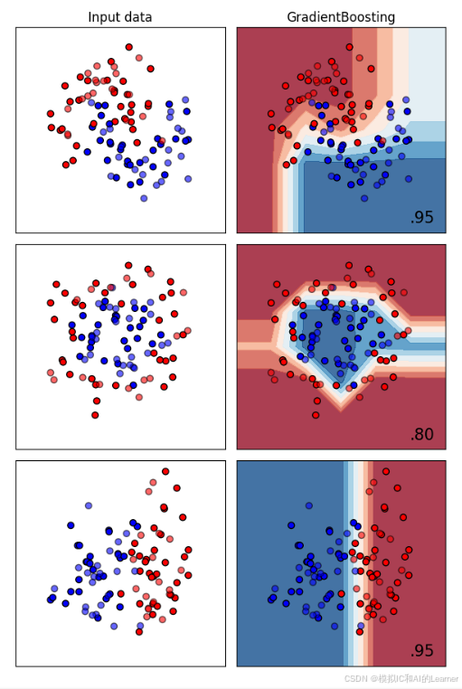
3、GradientBoosting(GBDT)——分类
#提升法——GradientBoosting(GBDT)——分类


import numpy as np
import matplotlib.pyplot as plt
from matplotlib.colors import ListedColormap
from sklearn.model_selection import train_test_split
from sklearn.preprocessing import StandardScaler
from sklearn.datasets import make_moons, make_circles, make_classification

from sklearn.ensemble import GradientBoostingClassifier


names = ["GradientBoosting"]


classifiers = [
    GradientBoostingClassifier(max_depth=5)
    ]

X, y = make_classification(n_features=2, n_redundant=0, n_informative=2,
                           random_state=1, n_clusters_per_class=1)


rng = np.random.RandomState(2)
X += 2 * rng.uniform(size=X.shape)
linearly_separable = (X, y)

datasets = [make_moons(noise=0.3, random_state=0),
            make_circles(noise=0.2, factor=0.5, random_state=1),
            linearly_separable
            ]

figure = plt.figure(figsize=(3*len(names)+3, 3*len(datasets)))
i = 1

# iterate over datasets
for ds_cnt, ds in enumerate(datasets):
    # preprocess dataset, split into training and test part
    X, y = ds
    X = StandardScaler().fit_transform(X)
    X_train, X_test, y_train, y_test = \
        train_test_split(X, y, test_size=.4, random_state=42)

    x_min, x_max = X[:, 0].min() - 1, X[:, 0].max() + 2
    y_min, y_max = X[:, 1].min() - 1, X[:, 1].max() + 1
    xx, yy = np.meshgrid(np.arange(x_min, x_max),
                         np.arange(y_min, y_max))

    # just plot the dataset first
    cm = plt.cm.RdBu
    cm_bright = ListedColormap(['#FF0000', '#0000FF'])
    ax = plt.subplot(len(datasets), len(classifiers) + 1, i)
    if ds_cnt == 0:
        ax.set_title("Input data")
    # Plot the training points
    ax.scatter(X_train[:, 0], X_train[:, 1], c=y_train, cmap=cm_bright,
               edgecolors='k')
    # Plot the testing points
    ax.scatter(X_test[:, 0], X_test[:, 1], c=y_test, cmap=cm_bright, alpha=0.6,
               edgecolors='k')
    ax.set_xlim(xx.min(), xx.max())
    ax.set_ylim(yy.min(), yy.max())
    ax.set_xticks(())
    ax.set_yticks(())
    i += 1

    # iterate over classifiers
    for name, clf in zip(names, classifiers):
        ax = plt.subplot(len(datasets), len(classifiers) + 1, i)
        clf.fit(X_train, y_train)
        score = clf.score(X_test, y_test)

        # Plot the decision boundary. For that, we will assign a color to each
        # point in the mesh [x_min, x_max]x[y_min, y_max].
        if hasattr(clf, "decision_function"):
            Z = clf.decision_function(np.c_[xx.ravel(), yy.ravel()])
        else:
            Z = clf.predict_proba(np.c_[xx.ravel(), yy.ravel()])[:, 1]

        # Put the result into a color plot
        Z = Z.reshape(xx.shape)
        ax.contourf(xx, yy, Z, cmap=cm, alpha=.8)

        # Plot the training points
        ax.scatter(X_train[:, 0], X_train[:, 1], c=y_train, cmap=cm_bright,
                   edgecolors='k')
        # Plot the testing points
        ax.scatter(X_test[:, 0], X_test[:, 1], c=y_test, cmap=cm_bright,
                   edgecolors='k', alpha=0.6)

        ax.set_xlim(xx.min(), xx.max())
        ax.set_ylim(yy.min(), yy.max())
        ax.set_xticks(())
        ax.set_yticks(())
        if ds_cnt == 0:
            ax.set_title(name)
        ax.text(xx.max() - .3, yy.min() + .3, ('%.2f' % score).lstrip('0'),
                size=15, horizontalalignment='right')
        i += 1

plt.tight_layout()
plt.show()
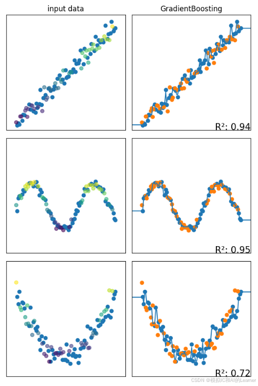
4、GradientBoosting(GBDT)——回归
#提升法——GradientBoosting(GBDT)——回归


import numpy as np
import matplotlib.pyplot as plt
from matplotlib.colors import ListedColormap
from sklearn.model_selection import train_test_split
from sklearn.preprocessing import StandardScaler
from sklearn.datasets import make_regression


from sklearn.ensemble import GradientBoostingRegressor

# 定义回归器名称和模型
names = ["GradientBoosting"]
regressors = [
     GradientBoostingRegressor()
     ]

# 生成数据集
# 数据集1:线性回归数据集: y = 2x + 1
X_lin = np.linspace(0, 10, 100)
y_lin = 2 * X_lin + 1 + np.random.normal(0, 1, size=100)
# 数据集2:非线性回归数据集(正弦关系): y = sin(x)
X_sin = np.linspace(0, 10, 100)
y_sin = np.sin(X_sin) + np.random.normal(0, 0.1, size=100)
# 数据集3:二次曲线回归数据集:y = 0.2x^2 - 2x + 5
X_quad = np.linspace(0, 10, 100)
y_quad = 0.2 * X_quad**2 - 2 * X_quad + 5 + np.random.normal(0, 0.5, size=100)

datasets = [(X_lin, y_lin), (X_sin, y_sin), (X_quad, y_quad)]

figure = plt.figure(figsize=(3*len(names)+3, 3*len(datasets)))
i = 1
h = 1  # 网格步长

# 遍历每个数据集
for ds_cnt, ds in enumerate(datasets):
    X, y = ds
    # 划分训练集和测试集
    X_train, X_test, y_train, y_test = train_test_split(X, y, test_size=0.4, random_state=42)

    # 定义网格边界
    x_min, x_max = X.min()-1 , X.max()+2
    y_min, y_max = y.min()-1 , y.max()+2
    xx, yy = np.meshgrid(np.arange(x_min, x_max, h),
                         np.arange(y_min, y_max, h))

    # 第一个子图:绘制原始数据(训练集和测试集)
    ax = plt.subplot(len(datasets), len(regressors) + 1, i)
    if ds_cnt == 0:
        ax.set_title("input data")
    sc = ax.scatter(X_train, y_train)
    ax.scatter(X_test, y_test, c=y_test,  alpha=0.6)
    ax.set_xlim(xx.min(), xx.max())
    ax.set_ylim(yy.min(), yy.max())
    ax.set_xticks(())
    ax.set_yticks(())

    i += 1

    # 遍历每个SVR模型
    for name, reg in zip(names, regressors):
        ax = plt.subplot(len(datasets), len(regressors) + 1, i)
        X_train = np.array(X_train).reshape(-1, 1)
        reg.fit(X_train,y_train)
        X_test = np.array(X_test).reshape(-1, 1)

        score = reg.score(X_test, y_test)  # R²得分


        # 绘制训练和测试数据点
        sc_train = ax.scatter(X_train, y_train)
        ax.scatter(X_test, y_test)
        ax.set_xlim(xx.min(), xx.max())
        ax.set_ylim(yy.min(), yy.max())
        ax.set_xticks(())
        ax.set_yticks(())
        if ds_cnt == 0:
            ax.set_title(name)
        ax.text(xx.max(), yy.min(), f'R²: {score:.2f}', size=15,
                horizontalalignment='right')
        #绘制回归线
        X_pic = np.linspace(xx.min(), xx.max(), int(10*(xx.max()-xx.min())))
        X_pic = np.array(X_pic).reshape(-1, 1)
        y_pic = reg.predict(X_pic)
        ax.plot(X_pic, y_pic)


        i += 1

plt.tight_layout()
plt.show()
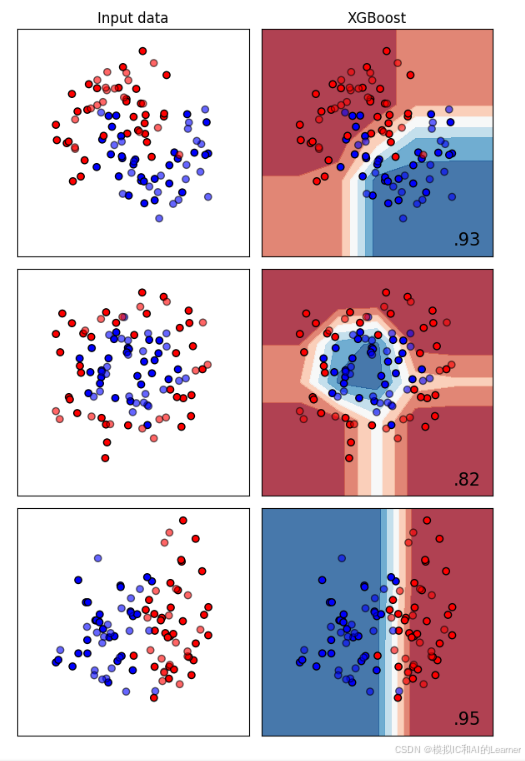
5、XGBoost——分类
#提升法——XGBoost——分类


import numpy as np
import matplotlib.pyplot as plt
from matplotlib.colors import ListedColormap
from sklearn.model_selection import train_test_split
from sklearn.preprocessing import StandardScaler
from sklearn.datasets import make_moons, make_circles, make_classification

import xgboost as xgb


names = ["XGBoost"]


classifiers = [
    xgb.XGBClassifier(objective='binary:logistic', eval_metric='logloss', max_depth=10, learning_rate=0.1, n_estimators=100, subsample=0.8)

    ]

X, y = make_classification(n_features=2, n_redundant=0, n_informative=2,
                           random_state=1, n_clusters_per_class=1)


rng = np.random.RandomState(2)
X += 2 * rng.uniform(size=X.shape)
linearly_separable = (X, y)

datasets = [make_moons(noise=0.3, random_state=0),
            make_circles(noise=0.2, factor=0.5, random_state=1),
            linearly_separable
            ]

figure = plt.figure(figsize=(3*len(names)+3, 3*len(datasets)))
i = 1

# iterate over datasets
for ds_cnt, ds in enumerate(datasets):
    # preprocess dataset, split into training and test part
    X, y = ds
    X = StandardScaler().fit_transform(X)
    X_train, X_test, y_train, y_test = \
        train_test_split(X, y, test_size=.4, random_state=42)

    x_min, x_max = X[:, 0].min() - 1, X[:, 0].max() + 2
    y_min, y_max = X[:, 1].min() - 1, X[:, 1].max() + 1
    xx, yy = np.meshgrid(np.arange(x_min, x_max),
                         np.arange(y_min, y_max))

    # just plot the dataset first
    cm = plt.cm.RdBu
    cm_bright = ListedColormap(['#FF0000', '#0000FF'])
    ax = plt.subplot(len(datasets), len(classifiers) + 1, i)
    if ds_cnt == 0:
        ax.set_title("Input data")
    # Plot the training points
    ax.scatter(X_train[:, 0], X_train[:, 1], c=y_train, cmap=cm_bright,
               edgecolors='k')
    # Plot the testing points
    ax.scatter(X_test[:, 0], X_test[:, 1], c=y_test, cmap=cm_bright, alpha=0.6,
               edgecolors='k')
    ax.set_xlim(xx.min(), xx.max())
    ax.set_ylim(yy.min(), yy.max())
    ax.set_xticks(())
    ax.set_yticks(())
    i += 1

    # iterate over classifiers
    for name, clf in zip(names, classifiers):
        ax = plt.subplot(len(datasets), len(classifiers) + 1, i)
        clf.fit(X_train, y_train)
        score = clf.score(X_test, y_test)

        # Plot the decision boundary. For that, we will assign a color to each
        # point in the mesh [x_min, x_max]x[y_min, y_max].
        if hasattr(clf, "decision_function"):
            Z = clf.decision_function(np.c_[xx.ravel(), yy.ravel()])
        else:
            Z = clf.predict_proba(np.c_[xx.ravel(), yy.ravel()])[:, 1]

        # Put the result into a color plot
        Z = Z.reshape(xx.shape)
        ax.contourf(xx, yy, Z, cmap=cm, alpha=.8)

        # Plot the training points
        ax.scatter(X_train[:, 0], X_train[:, 1], c=y_train, cmap=cm_bright,
                   edgecolors='k')
        # Plot the testing points
        ax.scatter(X_test[:, 0], X_test[:, 1], c=y_test, cmap=cm_bright,
                   edgecolors='k', alpha=0.6)

        ax.set_xlim(xx.min(), xx.max())
        ax.set_ylim(yy.min(), yy.max())
        ax.set_xticks(())
        ax.set_yticks(())
        if ds_cnt == 0:
            ax.set_title(name)
        ax.text(xx.max() - .3, yy.min() + .3, ('%.2f' % score).lstrip('0'),
                size=15, horizontalalignment='right')
        i += 1

plt.tight_layout()
plt.show()
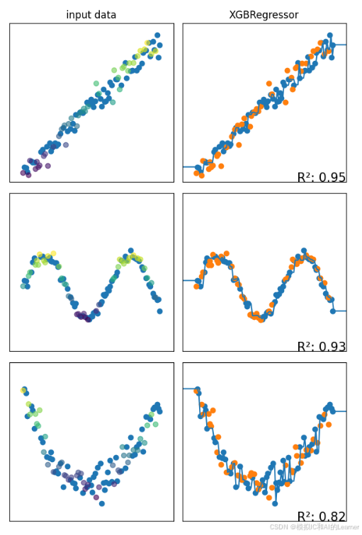
6、XGBoost——回归
#提升法——XGBoost——回归


import numpy as np
import matplotlib.pyplot as plt
from matplotlib.colors import ListedColormap
from sklearn.model_selection import train_test_split
from sklearn.preprocessing import StandardScaler
from sklearn.datasets import make_regression


import xgboost as xgb

# 定义回归器名称和模型
names = ["XGBRegressor"]
regressors = [
     xgb.XGBRegressor(objective='reg:squarederror', eval_metric='rmse', n_estimators=100)
     ]

# 生成数据集
# 数据集1:线性回归数据集: y = 2x + 1
X_lin = np.linspace(0, 10, 100)
y_lin = 2 * X_lin + 1 + np.random.normal(0, 1, size=100)
# 数据集2:非线性回归数据集(正弦关系): y = sin(x)
X_sin = np.linspace(0, 10, 100)
y_sin = np.sin(X_sin) + np.random.normal(0, 0.1, size=100)
# 数据集3:二次曲线回归数据集:y = 0.2x^2 - 2x + 5
X_quad = np.linspace(0, 10, 100)
y_quad = 0.2 * X_quad**2 - 2 * X_quad + 5 + np.random.normal(0, 0.5, size=100)

datasets = [(X_lin, y_lin), (X_sin, y_sin), (X_quad, y_quad)]

figure = plt.figure(figsize=(3*len(names)+3, 3*len(datasets)))
i = 1
h = 1  # 网格步长

# 遍历每个数据集
for ds_cnt, ds in enumerate(datasets):
    X, y = ds
    # 划分训练集和测试集
    X_train, X_test, y_train, y_test = train_test_split(X, y, test_size=0.4, random_state=42)

    # 定义网格边界
    x_min, x_max = X.min()-1 , X.max()+2
    y_min, y_max = y.min()-1 , y.max()+2
    xx, yy = np.meshgrid(np.arange(x_min, x_max, h),
                         np.arange(y_min, y_max, h))

    # 第一个子图:绘制原始数据(训练集和测试集)
    ax = plt.subplot(len(datasets), len(regressors) + 1, i)
    if ds_cnt == 0:
        ax.set_title("input data")
    sc = ax.scatter(X_train, y_train)
    ax.scatter(X_test, y_test, c=y_test,  alpha=0.6)
    ax.set_xlim(xx.min(), xx.max())
    ax.set_ylim(yy.min(), yy.max())
    ax.set_xticks(())
    ax.set_yticks(())

    i += 1

    # 遍历每个SVR模型
    for name, reg in zip(names, regressors):
        ax = plt.subplot(len(datasets), len(regressors) + 1, i)
        X_train = np.array(X_train).reshape(-1, 1)
        reg.fit(X_train,y_train)
        X_test = np.array(X_test).reshape(-1, 1)

        score = reg.score(X_test, y_test)  # R²得分


        # 绘制训练和测试数据点
        sc_train = ax.scatter(X_train, y_train)
        ax.scatter(X_test, y_test)
        ax.set_xlim(xx.min(), xx.max())
        ax.set_ylim(yy.min(), yy.max())
        ax.set_xticks(())
        ax.set_yticks(())
        if ds_cnt == 0:
            ax.set_title(name)
        ax.text(xx.max(), yy.min(), f'R²: {score:.2f}', size=15,
                horizontalalignment='right')
        #绘制回归线
        X_pic = np.linspace(xx.min(), xx.max(), int(10*(xx.max()-xx.min())))
        X_pic = np.array(X_pic).reshape(-1, 1)
        y_pic = reg.predict(X_pic)
        ax.plot(X_pic, y_pic)


        i += 1

plt.tight_layout()
plt.show()
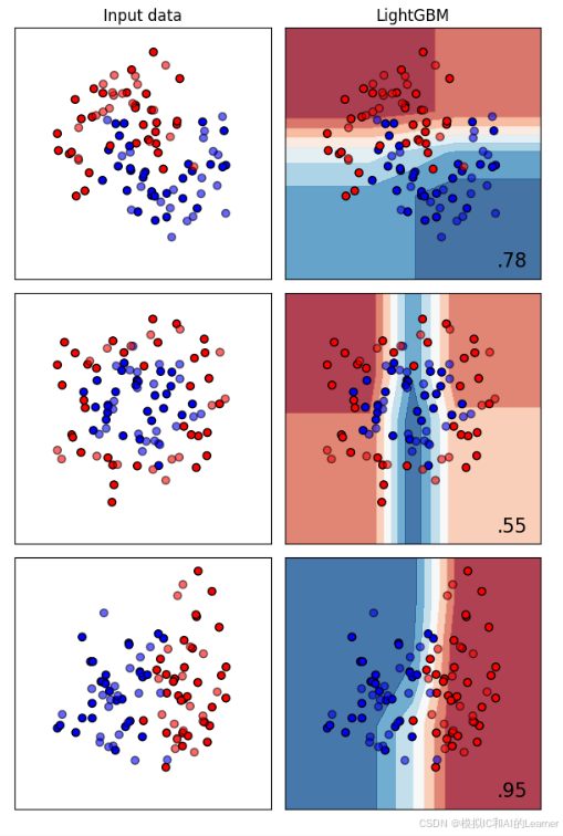
7、LightGBM——分类
对大规模数据效果好。
#提升法——LightGBM——分类


import numpy as np
import matplotlib.pyplot as plt
from matplotlib.colors import ListedColormap
from sklearn.model_selection import train_test_split
from sklearn.preprocessing import StandardScaler
from sklearn.datasets import make_moons, make_circles, make_classification

!pip install lightgbm
from lightgbm import LGBMClassifier


names = ["LightGBM"]


classifiers = [
    LGBMClassifier(num_leaves=31,learning_rate=0.1,n_estimators=100)

    ]

X, y = make_classification(n_features=2, n_redundant=0, n_informative=2,
                           random_state=1, n_clusters_per_class=1)


rng = np.random.RandomState(2)
X += 2 * rng.uniform(size=X.shape)
linearly_separable = (X, y)

datasets = [make_moons(noise=0.3, random_state=0),
            make_circles(noise=0.2, factor=0.5, random_state=1),
            linearly_separable
            ]

figure = plt.figure(figsize=(3*len(names)+3, 3*len(datasets)))
i = 1

# iterate over datasets
for ds_cnt, ds in enumerate(datasets):
    # preprocess dataset, split into training and test part
    X, y = ds
    X = StandardScaler().fit_transform(X)
    X_train, X_test, y_train, y_test = \
        train_test_split(X, y, test_size=.4, random_state=42)

    x_min, x_max = X[:, 0].min() - 1, X[:, 0].max() + 2
    y_min, y_max = X[:, 1].min() - 1, X[:, 1].max() + 1
    xx, yy = np.meshgrid(np.arange(x_min, x_max),
                         np.arange(y_min, y_max))

    # just plot the dataset first
    cm = plt.cm.RdBu
    cm_bright = ListedColormap(['#FF0000', '#0000FF'])
    ax = plt.subplot(len(datasets), len(classifiers) + 1, i)
    if ds_cnt == 0:
        ax.set_title("Input data")
    # Plot the training points
    ax.scatter(X_train[:, 0], X_train[:, 1], c=y_train, cmap=cm_bright,
               edgecolors='k')
    # Plot the testing points
    ax.scatter(X_test[:, 0], X_test[:, 1], c=y_test, cmap=cm_bright, alpha=0.6,
               edgecolors='k')
    ax.set_xlim(xx.min(), xx.max())
    ax.set_ylim(yy.min(), yy.max())
    ax.set_xticks(())
    ax.set_yticks(())
    i += 1

    # iterate over classifiers
    for name, clf in zip(names, classifiers):
        ax = plt.subplot(len(datasets), len(classifiers) + 1, i)
        clf.fit(X_train, y_train)
        score = clf.score(X_test, y_test)

        # Plot the decision boundary. For that, we will assign a color to each
        # point in the mesh [x_min, x_max]x[y_min, y_max].
        if hasattr(clf, "decision_function"):
            Z = clf.decision_function(np.c_[xx.ravel(), yy.ravel()])
        else:
            Z = clf.predict_proba(np.c_[xx.ravel(), yy.ravel()])[:, 1]

        # Put the result into a color plot
        Z = Z.reshape(xx.shape)
        ax.contourf(xx, yy, Z, cmap=cm, alpha=.8)

        # Plot the training points
        ax.scatter(X_train[:, 0], X_train[:, 1], c=y_train, cmap=cm_bright,
                   edgecolors='k')
        # Plot the testing points
        ax.scatter(X_test[:, 0], X_test[:, 1], c=y_test, cmap=cm_bright,
                   edgecolors='k', alpha=0.6)

        ax.set_xlim(xx.min(), xx.max())
        ax.set_ylim(yy.min(), yy.max())
        ax.set_xticks(())
        ax.set_yticks(())
        if ds_cnt == 0:
            ax.set_title(name)
        ax.text(xx.max() - .3, yy.min() + .3, ('%.2f' % score).lstrip('0'),
                size=15, horizontalalignment='right')
        i += 1

plt.tight_layout()
plt.show()
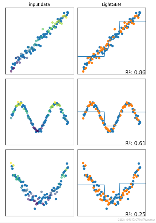
8、LightGBM——回归
#提升法——LightGBM——回归


import numpy as np
import matplotlib.pyplot as plt
from matplotlib.colors import ListedColormap
from sklearn.model_selection import train_test_split
from sklearn.preprocessing import StandardScaler
from sklearn.datasets import make_regression

!pip install lightgbm
from lightgbm import LGBMRegressor

# 定义回归器名称和模型
names = ["LightGBM"]
regressors = [
     LGBMRegressor(num_leaves=31, learning_rate=0.05, n_estimators=200, random_state=42)
     ]

# 生成数据集
# 数据集1:线性回归数据集: y = 2x + 1
X_lin = np.linspace(0, 10, 100)
y_lin = 2 * X_lin + 1 + np.random.normal(0, 1, size=100)
# 数据集2:非线性回归数据集(正弦关系): y = sin(x)
X_sin = np.linspace(0, 10, 100)
y_sin = np.sin(X_sin) + np.random.normal(0, 0.1, size=100)
# 数据集3:二次曲线回归数据集:y = 0.2x^2 - 2x + 5
X_quad = np.linspace(0, 10, 100)
y_quad = 0.2 * X_quad**2 - 2 * X_quad + 5 + np.random.normal(0, 0.5, size=100)

datasets = [(X_lin, y_lin), (X_sin, y_sin), (X_quad, y_quad)]

figure = plt.figure(figsize=(3*len(names)+3, 3*len(datasets)))
i = 1
h = 1  # 网格步长

# 遍历每个数据集
for ds_cnt, ds in enumerate(datasets):
    X, y = ds
    # 划分训练集和测试集
    X_train, X_test, y_train, y_test = train_test_split(X, y, test_size=0.4, random_state=42)

    # 定义网格边界
    x_min, x_max = X.min()-1 , X.max()+2
    y_min, y_max = y.min()-1 , y.max()+2
    xx, yy = np.meshgrid(np.arange(x_min, x_max, h),
                         np.arange(y_min, y_max, h))

    # 第一个子图:绘制原始数据(训练集和测试集)
    ax = plt.subplot(len(datasets), len(regressors) + 1, i)
    if ds_cnt == 0:
        ax.set_title("input data")
    sc = ax.scatter(X_train, y_train)
    ax.scatter(X_test, y_test, c=y_test,  alpha=0.6)
    ax.set_xlim(xx.min(), xx.max())
    ax.set_ylim(yy.min(), yy.max())
    ax.set_xticks(())
    ax.set_yticks(())

    i += 1

    # 遍历每个SVR模型
    for name, reg in zip(names, regressors):
        ax = plt.subplot(len(datasets), len(regressors) + 1, i)
        X_train = np.array(X_train).reshape(-1, 1)
        reg.fit(X_train,y_train)
        X_test = np.array(X_test).reshape(-1, 1)

        score = reg.score(X_test, y_test)  # R²得分


        # 绘制训练和测试数据点
        sc_train = ax.scatter(X_train, y_train)
        ax.scatter(X_test, y_test)
        ax.set_xlim(xx.min(), xx.max())
        ax.set_ylim(yy.min(), yy.max())
        ax.set_xticks(())
        ax.set_yticks(())
        if ds_cnt == 0:
            ax.set_title(name)
        ax.text(xx.max(), yy.min(), f'R²: {score:.2f}', size=15,
                horizontalalignment='right')
        #绘制回归线
        X_pic = np.linspace(xx.min(), xx.max(), int(10*(xx.max()-xx.min())))
        X_pic = np.array(X_pic).reshape(-1, 1)
        y_pic = reg.predict(X_pic)
        ax.plot(X_pic, y_pic)


        i += 1

plt.tight_layout()
plt.show()
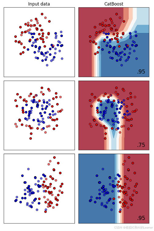
9、CatBoost——分类
CatBoost对类别型特征单列出来特殊处理。
其主要优势是能处理类别特征,并且具有出色的性能和高效性。
#提升法——CatBoost——分类


import numpy as np
import matplotlib.pyplot as plt
from matplotlib.colors import ListedColormap
from sklearn.model_selection import train_test_split
from sklearn.preprocessing import StandardScaler
from sklearn.datasets import make_moons, make_circles, make_classification

!pip install catboost
from catboost import CatBoostClassifier


names = ["CatBoost"]


classifiers = [
    CatBoostClassifier(iterations=500, depth=10, learning_rate=0.1, cat_features=[])

    ]

X, y = make_classification(n_features=2, n_redundant=0, n_informative=2,
                           random_state=1, n_clusters_per_class=1)


rng = np.random.RandomState(2)
X += 2 * rng.uniform(size=X.shape)
linearly_separable = (X, y)

datasets = [make_moons(noise=0.3, random_state=0),
            make_circles(noise=0.2, factor=0.5, random_state=1),
            linearly_separable
            ]

figure = plt.figure(figsize=(3*len(names)+3, 3*len(datasets)))
i = 1

# iterate over datasets
for ds_cnt, ds in enumerate(datasets):
    # preprocess dataset, split into training and test part
    X, y = ds
    X = StandardScaler().fit_transform(X)
    X_train, X_test, y_train, y_test = \
        train_test_split(X, y, test_size=.4, random_state=42)

    x_min, x_max = X[:, 0].min() - 1, X[:, 0].max() + 2
    y_min, y_max = X[:, 1].min() - 1, X[:, 1].max() + 1
    xx, yy = np.meshgrid(np.arange(x_min, x_max),
                         np.arange(y_min, y_max))

    # just plot the dataset first
    cm = plt.cm.RdBu
    cm_bright = ListedColormap(['#FF0000', '#0000FF'])
    ax = plt.subplot(len(datasets), len(classifiers) + 1, i)
    if ds_cnt == 0:
        ax.set_title("Input data")
    # Plot the training points
    ax.scatter(X_train[:, 0], X_train[:, 1], c=y_train, cmap=cm_bright,
               edgecolors='k')
    # Plot the testing points
    ax.scatter(X_test[:, 0], X_test[:, 1], c=y_test, cmap=cm_bright, alpha=0.6,
               edgecolors='k')
    ax.set_xlim(xx.min(), xx.max())
    ax.set_ylim(yy.min(), yy.max())
    ax.set_xticks(())
    ax.set_yticks(())
    i += 1

    # iterate over classifiers
    for name, clf in zip(names, classifiers):
        ax = plt.subplot(len(datasets), len(classifiers) + 1, i)
        clf.fit(X_train, y_train)
        score = clf.score(X_test, y_test)

        # Plot the decision boundary. For that, we will assign a color to each
        # point in the mesh [x_min, x_max]x[y_min, y_max].
        if hasattr(clf, "decision_function"):
            Z = clf.decision_function(np.c_[xx.ravel(), yy.ravel()])
        else:
            Z = clf.predict_proba(np.c_[xx.ravel(), yy.ravel()])[:, 1]

        # Put the result into a color plot
        Z = Z.reshape(xx.shape)
        ax.contourf(xx, yy, Z, cmap=cm, alpha=.8)

        # Plot the training points
        ax.scatter(X_train[:, 0], X_train[:, 1], c=y_train, cmap=cm_bright,
                   edgecolors='k')
        # Plot the testing points
        ax.scatter(X_test[:, 0], X_test[:, 1], c=y_test, cmap=cm_bright,
                   edgecolors='k', alpha=0.6)

        ax.set_xlim(xx.min(), xx.max())
        ax.set_ylim(yy.min(), yy.max())
        ax.set_xticks(())
        ax.set_yticks(())
        if ds_cnt == 0:
            ax.set_title(name)
        ax.text(xx.max() - .3, yy.min() + .3, ('%.2f' % score).lstrip('0'),
                size=15, horizontalalignment='right')
        i += 1

plt.tight_layout()
plt.show()
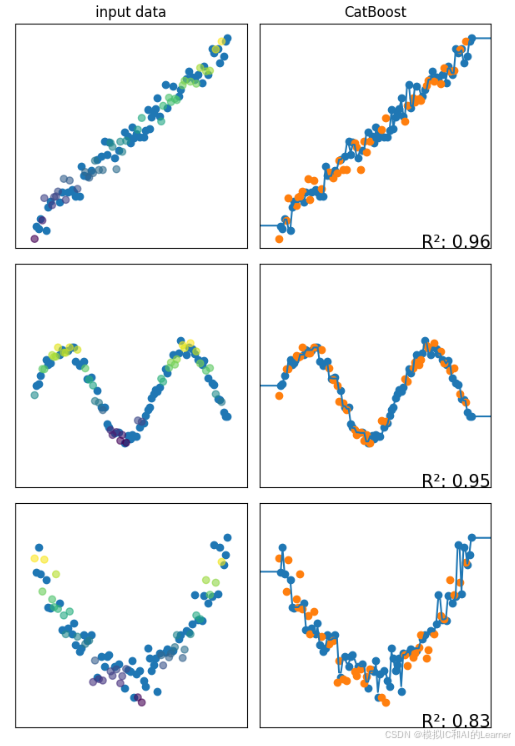
10、CatBoost——回归
#提升法——CatBoost——回归


import numpy as np
import matplotlib.pyplot as plt
from matplotlib.colors import ListedColormap
from sklearn.model_selection import train_test_split
from sklearn.preprocessing import StandardScaler
from sklearn.datasets import make_regression

!pip install catboost
from catboost import CatBoostRegressor

# 定义回归器名称和模型
names = ["CatBoost"]
regressors = [
     CatBoostRegressor(iterations=500, learning_rate=0.1, depth=6, cat_features=[])
     ]

# 生成数据集
# 数据集1:线性回归数据集: y = 2x + 1
X_lin = np.linspace(0, 10, 100)
y_lin = 2 * X_lin + 1 + np.random.normal(0, 1, size=100)
# 数据集2:非线性回归数据集(正弦关系): y = sin(x)
X_sin = np.linspace(0, 10, 100)
y_sin = np.sin(X_sin) + np.random.normal(0, 0.1, size=100)
# 数据集3:二次曲线回归数据集:y = 0.2x^2 - 2x + 5
X_quad = np.linspace(0, 10, 100)
y_quad = 0.2 * X_quad**2 - 2 * X_quad + 5 + np.random.normal(0, 0.5, size=100)

datasets = [(X_lin, y_lin), (X_sin, y_sin), (X_quad, y_quad)]

figure = plt.figure(figsize=(3*len(names)+3, 3*len(datasets)))
i = 1
h = 1  # 网格步长

# 遍历每个数据集
for ds_cnt, ds in enumerate(datasets):
    X, y = ds
    # 划分训练集和测试集
    X_train, X_test, y_train, y_test = train_test_split(X, y, test_size=0.4, random_state=42)

    # 定义网格边界
    x_min, x_max = X.min()-1 , X.max()+2
    y_min, y_max = y.min()-1 , y.max()+2
    xx, yy = np.meshgrid(np.arange(x_min, x_max, h),
                         np.arange(y_min, y_max, h))

    # 第一个子图:绘制原始数据(训练集和测试集)
    ax = plt.subplot(len(datasets), len(regressors) + 1, i)
    if ds_cnt == 0:
        ax.set_title("input data")
    sc = ax.scatter(X_train, y_train)
    ax.scatter(X_test, y_test, c=y_test,  alpha=0.6)
    ax.set_xlim(xx.min(), xx.max())
    ax.set_ylim(yy.min(), yy.max())
    ax.set_xticks(())
    ax.set_yticks(())

    i += 1

    # 遍历每个SVR模型
    for name, reg in zip(names, regressors):
        ax = plt.subplot(len(datasets), len(regressors) + 1, i)
        X_train = np.array(X_train).reshape(-1, 1)
        reg.fit(X_train,y_train)
        X_test = np.array(X_test).reshape(-1, 1)

        score = reg.score(X_test, y_test)  # R²得分


        # 绘制训练和测试数据点
        sc_train = ax.scatter(X_train, y_train)
        ax.scatter(X_test, y_test)
        ax.set_xlim(xx.min(), xx.max())
        ax.set_ylim(yy.min(), yy.max())
        ax.set_xticks(())
        ax.set_yticks(())
        if ds_cnt == 0:
            ax.set_title(name)
        ax.text(xx.max(), yy.min(), f'R²: {score:.2f}', size=15,
                horizontalalignment='right')
        #绘制回归线
        X_pic = np.linspace(xx.min(), xx.max(), int(10*(xx.max()-xx.min())))
        X_pic = np.array(X_pic).reshape(-1, 1)
        y_pic = reg.predict(X_pic)
        ax.plot(X_pic, y_pic)


        i += 1

plt.tight_layout()
plt.show()
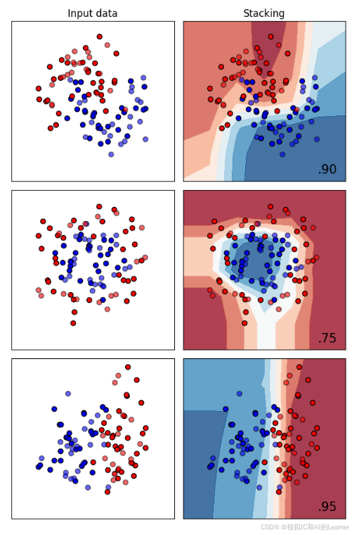
三、Stacking堆叠法
1、Stacking堆叠法——分类
#堆叠法——Stacking——分类


import numpy as np
import matplotlib.pyplot as plt
from matplotlib.colors import ListedColormap
from sklearn.model_selection import train_test_split
from sklearn.preprocessing import StandardScaler
from sklearn.datasets import make_moons, make_circles, make_classification


from sklearn.linear_model import LogisticRegression
from sklearn.tree import DecisionTreeClassifier
from sklearn.ensemble import RandomForestClassifier
from sklearn.metrics import accuracy_score
from sklearn.ensemble import StackingClassifier


names = ["Stacking"]


classifiers = [
    StackingClassifier(
        estimators=[('dt', DecisionTreeClassifier(max_depth=3)),('rf', RandomForestClassifier(n_estimators=10)),('lr', LogisticRegression(max_iter=1000))],
        final_estimator=LogisticRegression())

    ]

X, y = make_classification(n_features=2, n_redundant=0, n_informative=2,
                           random_state=1, n_clusters_per_class=1)


rng = np.random.RandomState(2)
X += 2 * rng.uniform(size=X.shape)
linearly_separable = (X, y)

datasets = [make_moons(noise=0.3, random_state=0),
            make_circles(noise=0.2, factor=0.5, random_state=1),
            linearly_separable
            ]

figure = plt.figure(figsize=(3*len(names)+3, 3*len(datasets)))
i = 1

# iterate over datasets
for ds_cnt, ds in enumerate(datasets):
    # preprocess dataset, split into training and test part
    X, y = ds
    X = StandardScaler().fit_transform(X)
    X_train, X_test, y_train, y_test = \
        train_test_split(X, y, test_size=.4, random_state=42)

    x_min, x_max = X[:, 0].min() - 1, X[:, 0].max() + 2
    y_min, y_max = X[:, 1].min() - 1, X[:, 1].max() + 1
    xx, yy = np.meshgrid(np.arange(x_min, x_max),
                         np.arange(y_min, y_max))

    # just plot the dataset first
    cm = plt.cm.RdBu
    cm_bright = ListedColormap(['#FF0000', '#0000FF'])
    ax = plt.subplot(len(datasets), len(classifiers) + 1, i)
    if ds_cnt == 0:
        ax.set_title("Input data")
    # Plot the training points
    ax.scatter(X_train[:, 0], X_train[:, 1], c=y_train, cmap=cm_bright,
               edgecolors='k')
    # Plot the testing points
    ax.scatter(X_test[:, 0], X_test[:, 1], c=y_test, cmap=cm_bright, alpha=0.6,
               edgecolors='k')
    ax.set_xlim(xx.min(), xx.max())
    ax.set_ylim(yy.min(), yy.max())
    ax.set_xticks(())
    ax.set_yticks(())
    i += 1

    # iterate over classifiers
    for name, clf in zip(names, classifiers):
        ax = plt.subplot(len(datasets), len(classifiers) + 1, i)
        clf.fit(X_train, y_train)
        score = clf.score(X_test, y_test)

        # Plot the decision boundary. For that, we will assign a color to each
        # point in the mesh [x_min, x_max]x[y_min, y_max].
        if hasattr(clf, "decision_function"):
            Z = clf.decision_function(np.c_[xx.ravel(), yy.ravel()])
        else:
            Z = clf.predict_proba(np.c_[xx.ravel(), yy.ravel()])[:, 1]

        # Put the result into a color plot
        Z = Z.reshape(xx.shape)
        ax.contourf(xx, yy, Z, cmap=cm, alpha=.8)

        # Plot the training points
        ax.scatter(X_train[:, 0], X_train[:, 1], c=y_train, cmap=cm_bright,
                   edgecolors='k')
        # Plot the testing points
        ax.scatter(X_test[:, 0], X_test[:, 1], c=y_test, cmap=cm_bright,
                   edgecolors='k', alpha=0.6)

        ax.set_xlim(xx.min(), xx.max())
        ax.set_ylim(yy.min(), yy.max())
        ax.set_xticks(())
        ax.set_yticks(())
        if ds_cnt == 0:
            ax.set_title(name)
        ax.text(xx.max() - .3, yy.min() + .3, ('%.2f' % score).lstrip('0'),
                size=15, horizontalalignment='right')
        i += 1

plt.tight_layout()
plt.show()
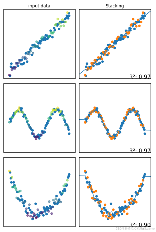
2、Stacking堆叠法——回归
#提升法——Stacking——回归


import numpy as np
import matplotlib.pyplot as plt
from matplotlib.colors import ListedColormap
from sklearn.model_selection import train_test_split
from sklearn.preprocessing import StandardScaler
from sklearn.datasets import make_regression

from sklearn.linear_model import LinearRegression
from sklearn.tree import DecisionTreeRegressor
from sklearn.ensemble import RandomForestRegressor
from sklearn.metrics import mean_squared_error
from sklearn.ensemble import StackingRegressor

# 定义回归器名称和模型
names = ["Stacking"]
regressors = [
     StackingRegressor(estimators=[('lr', LinearRegression()),('dt', DecisionTreeRegressor()),('rf', RandomForestRegressor())],
                       final_estimator=LinearRegression())
     ]

# 生成数据集
# 数据集1:线性回归数据集: y = 2x + 1
X_lin = np.linspace(0, 10, 100)
y_lin = 2 * X_lin + 1 + np.random.normal(0, 1, size=100)
# 数据集2:非线性回归数据集(正弦关系): y = sin(x)
X_sin = np.linspace(0, 10, 100)
y_sin = np.sin(X_sin) + np.random.normal(0, 0.1, size=100)
# 数据集3:二次曲线回归数据集:y = 0.2x^2 - 2x + 5
X_quad = np.linspace(0, 10, 100)
y_quad = 0.2 * X_quad**2 - 2 * X_quad + 5 + np.random.normal(0, 0.5, size=100)

datasets = [(X_lin, y_lin), (X_sin, y_sin), (X_quad, y_quad)]

figure = plt.figure(figsize=(3*len(names)+3, 3*len(datasets)))
i = 1
h = 1  # 网格步长

# 遍历每个数据集
for ds_cnt, ds in enumerate(datasets):
    X, y = ds
    # 划分训练集和测试集
    X_train, X_test, y_train, y_test = train_test_split(X, y, test_size=0.4, random_state=42)

    # 定义网格边界
    x_min, x_max = X.min()-1 , X.max()+2
    y_min, y_max = y.min()-1 , y.max()+2
    xx, yy = np.meshgrid(np.arange(x_min, x_max, h),
                         np.arange(y_min, y_max, h))

    # 第一个子图:绘制原始数据(训练集和测试集)
    ax = plt.subplot(len(datasets), len(regressors) + 1, i)
    if ds_cnt == 0:
        ax.set_title("input data")
    sc = ax.scatter(X_train, y_train)
    ax.scatter(X_test, y_test, c=y_test,  alpha=0.6)
    ax.set_xlim(xx.min(), xx.max())
    ax.set_ylim(yy.min(), yy.max())
    ax.set_xticks(())
    ax.set_yticks(())

    i += 1

    # 遍历每个SVR模型
    for name, reg in zip(names, regressors):
        ax = plt.subplot(len(datasets), len(regressors) + 1, i)
        X_train = np.array(X_train).reshape(-1, 1)
        reg.fit(X_train,y_train)
        X_test = np.array(X_test).reshape(-1, 1)

        score = reg.score(X_test, y_test)  # R²得分


        # 绘制训练和测试数据点
        sc_train = ax.scatter(X_train, y_train)
        ax.scatter(X_test, y_test)
        ax.set_xlim(xx.min(), xx.max())
        ax.set_ylim(yy.min(), yy.max())
        ax.set_xticks(())
        ax.set_yticks(())
        if ds_cnt == 0:
            ax.set_title(name)
        ax.text(xx.max(), yy.min(), f'R²: {score:.2f}', size=15,
                horizontalalignment='right')
        #绘制回归线
        X_pic = np.linspace(xx.min(), xx.max(), int(10*(xx.max()-xx.min())))
        X_pic = np.array(X_pic).reshape(-1, 1)
        y_pic = reg.predict(X_pic)
        ax.plot(X_pic, y_pic)


        i += 1

plt.tight_layout()
plt.show()
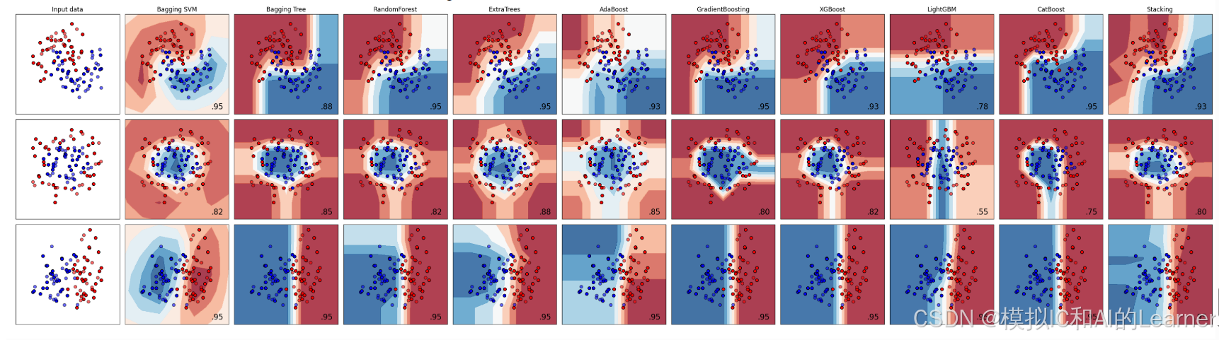
四、集成学习(总)
1、集成学习(总)——分类
#集成学习(总)——分类


import numpy as np
import matplotlib.pyplot as plt
from matplotlib.colors import ListedColormap
from sklearn.model_selection import train_test_split
from sklearn.preprocessing import StandardScaler
from sklearn.datasets import make_moons, make_circles, make_classification


from sklearn.svm import SVC
from sklearn.ensemble import BaggingClassifier
from sklearn.ensemble import RandomForestClassifier
from sklearn.ensemble import ExtraTreesClassifier
from sklearn.ensemble import StackingClassifier
from sklearn.ensemble import AdaBoostClassifier
from sklearn.ensemble import GradientBoostingClassifier
import xgboost as xgb
!pip install lightgbm
from lightgbm import LGBMClassifier
!pip install catboost
from catboost import CatBoostClassifier
from sklearn.linear_model import LogisticRegression
from sklearn.tree import DecisionTreeClassifier
from sklearn.ensemble import RandomForestClassifier
from sklearn.metrics import accuracy_score
from sklearn.ensemble import StackingClassifier


names = ["Bagging SVM","Bagging Tree","RandomForest","ExtraTrees","AdaBoost","GradientBoosting","XGBoost","LightGBM","CatBoost","Stacking"]


classifiers = [
    BaggingClassifier(estimator=SVC(), n_estimators=10, random_state=0),
    BaggingClassifier(estimator=None, n_estimators=10, random_state=0), #估计器默认是决策树
    RandomForestClassifier(max_depth=5, n_estimators=100, max_features=1),
    ExtraTreesClassifier(max_depth=5, n_estimators=100, random_state=0),
    AdaBoostClassifier(),
    GradientBoostingClassifier(max_depth=5),
    xgb.XGBClassifier(objective='binary:logistic', eval_metric='logloss', max_depth=10, learning_rate=0.1, n_estimators=100, subsample=0.8),
    LGBMClassifier(num_leaves=31,learning_rate=0.1,n_estimators=100),
    CatBoostClassifier(iterations=500, depth=10, learning_rate=0.1, cat_features=[]),
    StackingClassifier(
        estimators=[('dt', DecisionTreeClassifier(max_depth=3)),('rf', RandomForestClassifier(n_estimators=10)),('lr', LogisticRegression(max_iter=1000))],
        final_estimator=LogisticRegression())

    ]

X, y = make_classification(n_features=2, n_redundant=0, n_informative=2,
                           random_state=1, n_clusters_per_class=1)


rng = np.random.RandomState(2)
X += 2 * rng.uniform(size=X.shape)
linearly_separable = (X, y)

datasets = [make_moons(noise=0.3, random_state=0),
            make_circles(noise=0.2, factor=0.5, random_state=1),
            linearly_separable
            ]

figure = plt.figure(figsize=(3*len(names)+3, 3*len(datasets)))
i = 1

# iterate over datasets
for ds_cnt, ds in enumerate(datasets):
    # preprocess dataset, split into training and test part
    X, y = ds
    X = StandardScaler().fit_transform(X)
    X_train, X_test, y_train, y_test = \
        train_test_split(X, y, test_size=.4, random_state=42)

    x_min, x_max = X[:, 0].min() - 1, X[:, 0].max() + 2
    y_min, y_max = X[:, 1].min() - 1, X[:, 1].max() + 1
    xx, yy = np.meshgrid(np.arange(x_min, x_max),
                         np.arange(y_min, y_max))

    # just plot the dataset first
    cm = plt.cm.RdBu
    cm_bright = ListedColormap(['#FF0000', '#0000FF'])
    ax = plt.subplot(len(datasets), len(classifiers) + 1, i)
    if ds_cnt == 0:
        ax.set_title("Input data")
    # Plot the training points
    ax.scatter(X_train[:, 0], X_train[:, 1], c=y_train, cmap=cm_bright,
               edgecolors='k')
    # Plot the testing points
    ax.scatter(X_test[:, 0], X_test[:, 1], c=y_test, cmap=cm_bright, alpha=0.6,
               edgecolors='k')
    ax.set_xlim(xx.min(), xx.max())
    ax.set_ylim(yy.min(), yy.max())
    ax.set_xticks(())
    ax.set_yticks(())
    i += 1

    # iterate over classifiers
    for name, clf in zip(names, classifiers):
        ax = plt.subplot(len(datasets), len(classifiers) + 1, i)
        clf.fit(X_train, y_train)
        score = clf.score(X_test, y_test)

        # Plot the decision boundary. For that, we will assign a color to each
        # point in the mesh [x_min, x_max]x[y_min, y_max].
        if hasattr(clf, "decision_function"):
            Z = clf.decision_function(np.c_[xx.ravel(), yy.ravel()])
        else:
            Z = clf.predict_proba(np.c_[xx.ravel(), yy.ravel()])[:, 1]

        # Put the result into a color plot
        Z = Z.reshape(xx.shape)
        ax.contourf(xx, yy, Z, cmap=cm, alpha=.8)

        # Plot the training points
        ax.scatter(X_train[:, 0], X_train[:, 1], c=y_train, cmap=cm_bright,
                   edgecolors='k')
        # Plot the testing points
        ax.scatter(X_test[:, 0], X_test[:, 1], c=y_test, cmap=cm_bright,
                   edgecolors='k', alpha=0.6)

        ax.set_xlim(xx.min(), xx.max())
        ax.set_ylim(yy.min(), yy.max())
        ax.set_xticks(())
        ax.set_yticks(())
        if ds_cnt == 0:
            ax.set_title(name)
        ax.text(xx.max() - .3, yy.min() + .3, ('%.2f' % score).lstrip('0'),
                size=15, horizontalalignment='right')
        i += 1

plt.tight_layout()
plt.show()
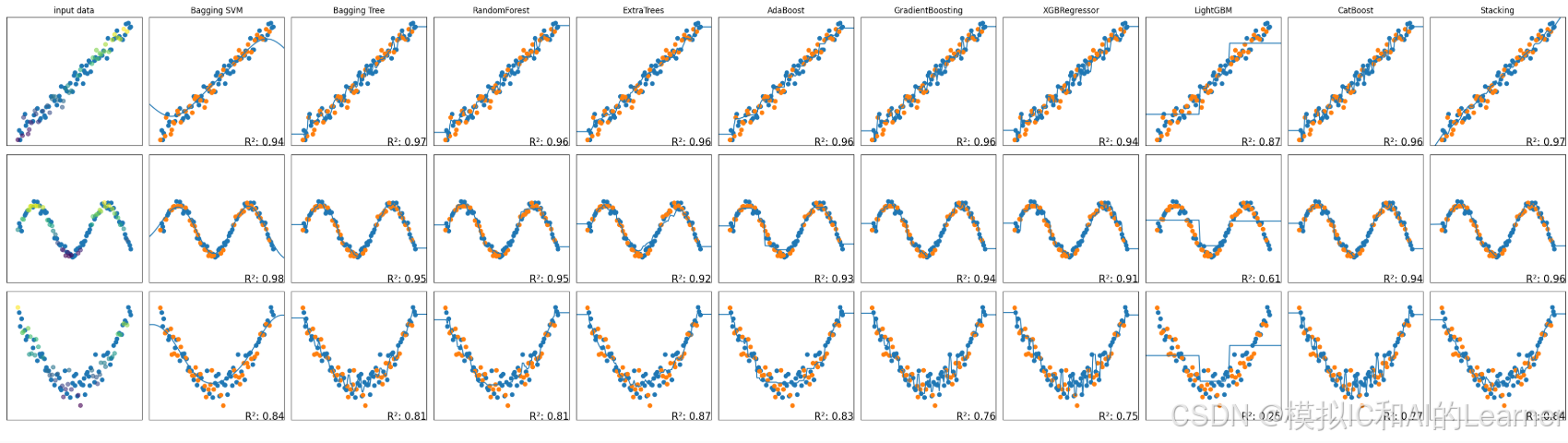
2、集成学习(总)——回归
#集成学习(总)——回归


import numpy as np
import matplotlib.pyplot as plt
from matplotlib.colors import ListedColormap
from sklearn.model_selection import train_test_split
from sklearn.preprocessing import StandardScaler
from sklearn.datasets import make_regression


from sklearn.svm import SVR
from sklearn.ensemble import BaggingRegressor
from sklearn.ensemble import RandomForestRegressor
from sklearn.ensemble import ExtraTreesRegressor
from sklearn.ensemble import AdaBoostRegressor
from sklearn.ensemble import GradientBoostingRegressor
import xgboost as xgb
!pip install lightgbm
from lightgbm import LGBMRegressor
!pip install catboost
from catboost import CatBoostRegressor
from sklearn.linear_model import LinearRegression
from sklearn.tree import DecisionTreeRegressor
from sklearn.ensemble import RandomForestRegressor
from sklearn.metrics import mean_squared_error
from sklearn.ensemble import StackingRegressor


# 定义回归器名称和模型
names = ["Bagging SVM", "Bagging Tree","RandomForest","ExtraTrees","AdaBoost","GradientBoosting","XGBRegressor","LightGBM","CatBoost","Stacking"]
regressors = [
    BaggingRegressor(estimator=SVR(), n_estimators=10, random_state=0),
    BaggingRegressor(estimator=None, n_estimators=10, random_state=0),
    RandomForestRegressor(max_depth=5, n_estimators=10, max_features=1),
    ExtraTreesRegressor(max_depth=5, n_estimators=10, random_state=0),
    AdaBoostRegressor(random_state=0, n_estimators=100),
    GradientBoostingRegressor(),
    xgb.XGBRegressor(objective='reg:squarederror', eval_metric='rmse', n_estimators=100),
    LGBMRegressor(num_leaves=31, learning_rate=0.05, n_estimators=200, random_state=42),
    CatBoostRegressor(iterations=500, learning_rate=0.1, depth=6, cat_features=[]),
    StackingRegressor(estimators=[('lr', LinearRegression()),('dt', DecisionTreeRegressor()),('rf', RandomForestRegressor())],
                       final_estimator=LinearRegression())
     ]

# 生成数据集
# 数据集1:线性回归数据集: y = 2x + 1
X_lin = np.linspace(0, 10, 100)
y_lin = 2 * X_lin + 1 + np.random.normal(0, 1, size=100)
# 数据集2:非线性回归数据集(正弦关系): y = sin(x)
X_sin = np.linspace(0, 10, 100)
y_sin = np.sin(X_sin) + np.random.normal(0, 0.1, size=100)
# 数据集3:二次曲线回归数据集:y = 0.2x^2 - 2x + 5
X_quad = np.linspace(0, 10, 100)
y_quad = 0.2 * X_quad**2 - 2 * X_quad + 5 + np.random.normal(0, 0.5, size=100)

datasets = [(X_lin, y_lin), (X_sin, y_sin), (X_quad, y_quad)]

figure = plt.figure(figsize=(3*len(names)+3, 3*len(datasets)))
i = 1
h = 1  # 网格步长

# 遍历每个数据集
for ds_cnt, ds in enumerate(datasets):
    X, y = ds
    # 划分训练集和测试集
    X_train, X_test, y_train, y_test = train_test_split(X, y, test_size=0.4, random_state=42)

    # 定义网格边界
    x_min, x_max = X.min()-1 , X.max()+2
    y_min, y_max = y.min()-1 , y.max()+2
    xx, yy = np.meshgrid(np.arange(x_min, x_max, h),
                         np.arange(y_min, y_max, h))

    # 第一个子图:绘制原始数据(训练集和测试集)
    ax = plt.subplot(len(datasets), len(regressors) + 1, i)
    if ds_cnt == 0:
        ax.set_title("input data")
    sc = ax.scatter(X_train, y_train)
    ax.scatter(X_test, y_test, c=y_test,  alpha=0.6)
    ax.set_xlim(xx.min(), xx.max())
    ax.set_ylim(yy.min(), yy.max())
    ax.set_xticks(())
    ax.set_yticks(())

    i += 1

    # 遍历每个SVR模型
    for name, reg in zip(names, regressors):
        ax = plt.subplot(len(datasets), len(regressors) + 1, i)
        X_train = np.array(X_train).reshape(-1, 1)
        reg.fit(X_train,y_train)
        X_test = np.array(X_test).reshape(-1, 1)

        score = reg.score(X_test, y_test)  # R²得分


        # 绘制训练和测试数据点
        sc_train = ax.scatter(X_train, y_train)
        ax.scatter(X_test, y_test)
        ax.set_xlim(xx.min(), xx.max())
        ax.set_ylim(yy.min(), yy.max())
        ax.set_xticks(())
        ax.set_yticks(())
        if ds_cnt == 0:
            ax.set_title(name)
        ax.text(xx.max(), yy.min(), f'R²: {score:.2f}', size=15,
                horizontalalignment='right')
        #绘制回归线
        X_pic = np.linspace(xx.min(), xx.max(), int(10*(xx.max()-xx.min())))
        X_pic = np.array(X_pic).reshape(-1, 1)
        y_pic = reg.predict(X_pic)
        ax.plot(X_pic, y_pic)


        i += 1

plt.tight_layout()
plt.show()


 被折叠的 条评论
为什么被折叠?
被折叠的 条评论
为什么被折叠?
 到【灌水乐园】发言


