【机器学习chp3代码示例】Fisher线性判别，感知机，最小平方误差分类器，广义线性判别函数，分段线性判别函数，最小距离分类器，CART树-优快云博客

Iris 数据集。该数据集包含 150 个样本、4 个特征（花萼长度，花萼宽度，花瓣长度，花瓣宽度），3种类别，由于数据集的规模较小且特征较为简单，Iris 数据集是机器学习学习者常用的入门数据集。它可以用来练习数据预处理、特征选择和分类算法的应用，尤其适用于线性和非线性分类算法的比较。我们可以将其简化为二分类问题，以便使用 Fisher 线性判别。
Wine 数据集。该数据集共有178个样本， 13 个特征（如酒的各类化学成分）以及 3 个不同类别（对应 3 种不同的葡萄酒）。Wine 数据集常用于评估分类算法，尤其是针对多类别分类任务。它的数据特征和类别之间有着较强的区分度，可以使用该数据集练习对特征进行降维（例如PCA）、数据标准化以及使用各种分类模型（例如逻辑回归、支持向量机等）。由于数据集的特征较多且有较强的区分性，这使得它成为了评估各种分类模型（尤其是基于特征选择的模型）性能的好选择。我们将把它转化为二分类问题来应用 Fisher 线性判别。
Breast Cancer Wisconsin 乳腺癌数据集。数据集共包含569个样本，其中有2个类别标签，这个数据集数据集包含 30 个特征（如细胞的对比度、纹理、平滑度等），用于描述肿瘤细胞的不同方面。该数据集常用于二分类任务，尤其是在医学诊断中的应用。它是用于测试分类器在处理不平衡数据（例如良性样本较多的情况下）的表现的一个很好的例子。除了分类任务外，乳腺癌数据集还常用于特征选择和模型评估。由于该数据集是医学领域的经典数据集之一，广泛应用于医学图像分析、机器学习方法的教学和开发，以及癌症诊断模型的验证。是二分类问题，包含了对乳腺癌细胞的各种特征测量，目标是通过特征判断癌症是良性（benign）还是恶性（malignant）。

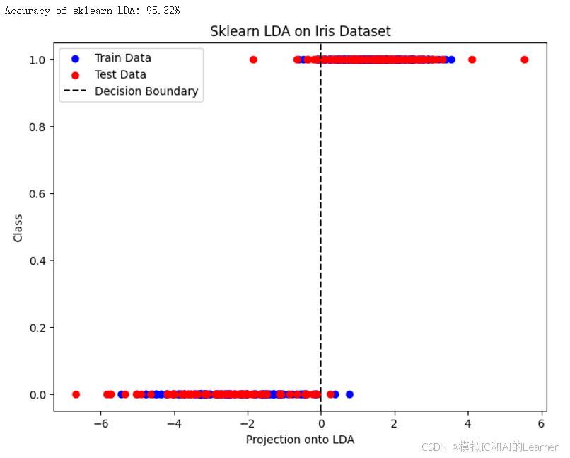
（1）Python代码——示例1——鸢尾花分类——Fisher LDA

import numpy as np
import matplotlib.pyplot as plt
from sklearn import datasets
from sklearn.model_selection import train_test_split
from sklearn.preprocessing import StandardScaler
from sklearn.metrics import accuracy_score

# 1. 加载Iris数据集
iris = datasets.load_iris()
X = iris.data
y = iris.target

# 只选择类别0和1，简化为二分类问题
X = X[y != 2]
y = y[y != 2]

# 2. 标准化特征数据
scaler = StandardScaler()
X = scaler.fit_transform(X)

# 3. 划分训练集和测试集
X_train, X_test, y_train, y_test = train_test_split(X, y, test_size=0.3, random_state=42)

# 4. Fisher线性判别（LDA）的实现

class FisherLDA:
    def __init__(self):
        self.w = None
        self.mu1 = None
        self.mu2 = None
        self.Sw = None
        self.Sb = None
        
    def fit(self, X, y):
        # 类别1和类别2的样本
        X1 = X[y == 0]
        X2 = X[y == 1]
        
        # 计算类别1和类别2的均值
        self.mu1 = np.mean(X1, axis=0)
        self.mu2 = np.mean(X2, axis=0)
        
        # 计算类内散度矩阵 Sw
        self.Sw = np.cov(X1.T) * (len(X1) - 1) + np.cov(X2.T) * (len(X2) - 1)
        
        # 计算类间散度矩阵 Sb
        self.Sb = np.outer(self.mu1 - self.mu2, self.mu1 - self.mu2)
        
        # 计算最佳投影方向 w
        self.w = np.linalg.inv(self.Sw).dot(self.mu1 - self.mu2)
        
    def transform(self, X):
        # 将数据投影到 w 上
        return X.dot(self.w)
    
    def predict(self, X):
        # 将测试数据投影并分类
        X_proj = self.transform(X)
        return np.where(X_proj > 0, 0, 1)

# 5. 创建Fisher LDA模型并进行训练
lda = FisherLDA()
lda.fit(X_train, y_train)

# 6. 在测试集上进行预测
y_pred = lda.predict(X_test)

# 7. 计算准确率
accuracy = accuracy_score(y_test, y_pred)
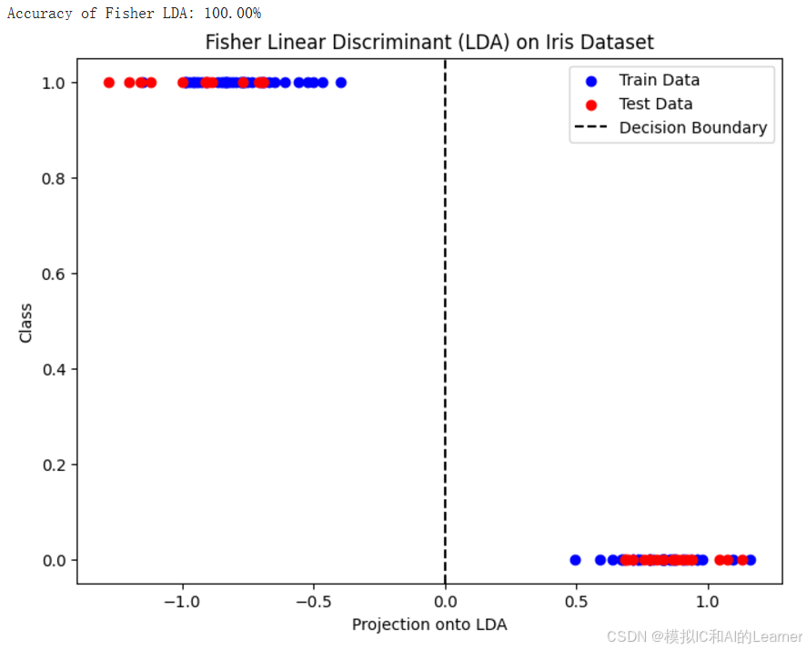
print(f"Accuracy of Fisher LDA: {accuracy * 100:.2f}%")

# 8. 可视化：将投影到LDA的1维数据
X_train_proj = lda.transform(X_train)
X_test_proj = lda.transform(X_test)

plt.figure(figsize=(8, 6))
plt.scatter(X_train_proj, y_train, color='blue', label='Train Data')
plt.scatter(X_test_proj, y_test, color='red', label='Test Data')
plt.axvline(x=0, color='black', linestyle='--', label='Decision Boundary')
plt.xlabel('Projection onto LDA')
plt.ylabel('Class')
plt.legend()
plt.title('Fisher Linear Discriminant (LDA) on Iris Dataset')
plt.show()

输出结果为：

（2）Python代码——示例1——鸢尾花分类——sklearn中的LDA

import numpy as np
import matplotlib.pyplot as plt
from sklearn import datasets
from sklearn.model_selection import train_test_split
from sklearn.preprocessing import StandardScaler
from sklearn.metrics import accuracy_score
from sklearn.discriminant_analysis import LinearDiscriminantAnalysis

# 1. 加载Iris数据集
iris = datasets.load_iris()
X = iris.data
y = iris.target

# 只选择类别0和1，简化为二分类问题
X = X[y != 2]
y = y[y != 2]

# 2. 标准化特征数据
scaler = StandardScaler()
X = scaler.fit_transform(X)

# 3. 划分训练集和测试集
X_train, X_test, y_train, y_test = train_test_split(X, y, test_size=0.3, random_state=42)

# 4. 使用sklearn中的LDA模型
lda = LinearDiscriminantAnalysis()

# 5. 训练LDA模型
lda.fit(X_train, y_train)

# 6. 在测试集上进行预测
y_pred = lda.predict(X_test)

# 7. 计算准确率
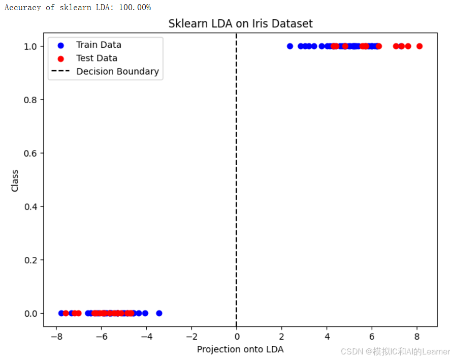
accuracy = accuracy_score(y_test, y_pred)
print(f"Accuracy of sklearn LDA: {accuracy * 100:.2f}%")

# 8. 可视化：将投影到LDA的1维数据
X_train_proj = lda.transform(X_train)
X_test_proj = lda.transform(X_test)

plt.figure(figsize=(8, 6))
plt.scatter(X_train_proj, y_train, color='blue', label='Train Data')
plt.scatter(X_test_proj, y_test, color='red', label='Test Data')
plt.axvline(x=0, color='black', linestyle='--', label='Decision Boundary')
plt.xlabel('Projection onto LDA')
plt.ylabel('Class')
plt.legend()
plt.title('Sklearn LDA on Iris Dataset')
plt.show()

输出结果为：

（3）Python代码——示例2——wine数据集分类——Fisher LDA

import numpy as np
import matplotlib.pyplot as plt
from sklearn import datasets
from sklearn.model_selection import train_test_split
from sklearn.preprocessing import StandardScaler
from sklearn.metrics import accuracy_score

# 1. 加载Wine数据集
wine = datasets.load_wine()
X = wine.data
y = wine.target

# 只选择类别0和类别1，简化为二分类问题
X = X[y != 2]
y = y[y != 2]

# 2. 标准化特征数据
scaler = StandardScaler()
X = scaler.fit_transform(X)

# 3. 划分训练集和测试集
X_train, X_test, y_train, y_test = train_test_split(X, y, test_size=0.3, random_state=42)

# 4. Fisher线性判别（LDA）的实现

class FisherLDA:
    def __init__(self):
        self.w = None
        self.mu1 = None
        self.mu2 = None
        self.Sw = None
        self.Sb = None
        
    def fit(self, X, y):
        # 类别1和类别2的样本
        X1 = X[y == 0]
        X2 = X[y == 1]
        
        # 计算类别1和类别2的均值
        self.mu1 = np.mean(X1, axis=0)
        self.mu2 = np.mean(X2, axis=0)
        
        # 计算类内散度矩阵 Sw
        self.Sw = np.cov(X1.T) * (len(X1) - 1) + np.cov(X2.T) * (len(X2) - 1)
        
        # 计算类间散度矩阵 Sb
        self.Sb = np.outer(self.mu1 - self.mu2, self.mu1 - self.mu2)
        
        # 计算最佳投影方向 w
        self.w = np.linalg.inv(self.Sw).dot(self.mu1 - self.mu2)
        
    def transform(self, X):
        # 将数据投影到 w 上
        return X.dot(self.w)
    
    def predict(self, X):
        # 将测试数据投影并分类
        X_proj = self.transform(X)
        return np.where(X_proj > 0, 0, 1)

# 5. 创建Fisher LDA模型并进行训练
lda = FisherLDA()
lda.fit(X_train, y_train)

# 6. 在测试集上进行预测
y_pred = lda.predict(X_test)

# 7. 计算准确率
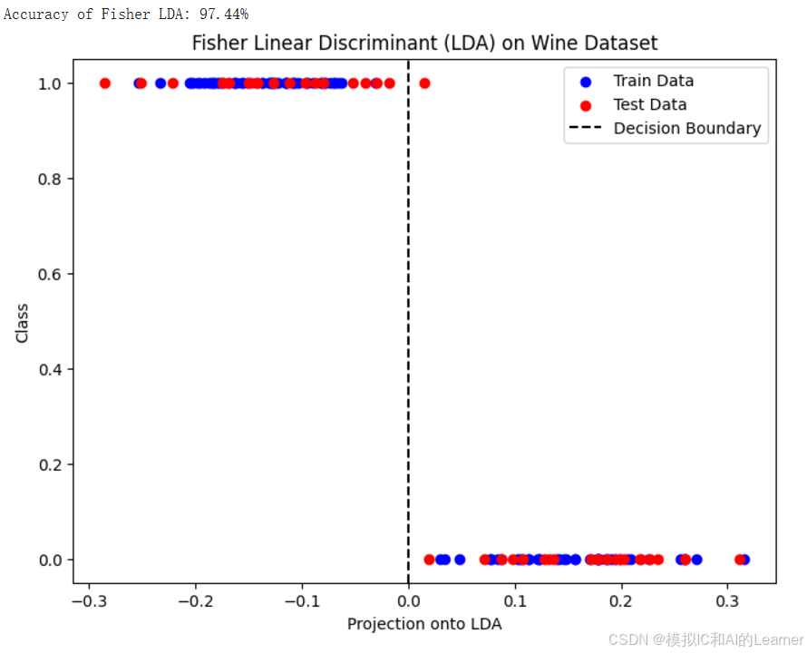
accuracy = accuracy_score(y_test, y_pred)
print(f"Accuracy of Fisher LDA: {accuracy * 100:.2f}%")

# 8. 可视化：将投影到LDA的1维数据
X_train_proj = lda.transform(X_train)
X_test_proj = lda.transform(X_test)

plt.figure(figsize=(8, 6))
plt.scatter(X_train_proj, y_train, color='blue', label='Train Data')
plt.scatter(X_test_proj, y_test, color='red', label='Test Data')
plt.axvline(x=0, color='black', linestyle='--', label='Decision Boundary')
plt.xlabel('Projection onto LDA')
plt.ylabel('Class')
plt.legend()
plt.title('Fisher Linear Discriminant (LDA) on Wine Dataset')
plt.show()

输出结果为：

（4）Python代码——示例2——wine数据集分类——sklearn中的LDA

import numpy as np
import matplotlib.pyplot as plt
from sklearn import datasets
from sklearn.model_selection import train_test_split
from sklearn.preprocessing import StandardScaler
from sklearn.metrics import accuracy_score
from sklearn.discriminant_analysis import LinearDiscriminantAnalysis

# 1. 加载Wine数据集
wine = datasets.load_wine()
X = wine.data
y = wine.target

# 只选择类别0和类别1，简化为二分类问题
X = X[y != 2]
y = y[y != 2]

# 2. 标准化特征数据
scaler = StandardScaler()
X = scaler.fit_transform(X)

# 3. 划分训练集和测试集
X_train, X_test, y_train, y_test = train_test_split(X, y, test_size=0.3, random_state=42)

# 4. 使用sklearn中的LDA模型
lda = LinearDiscriminantAnalysis()

# 5. 训练LDA模型
lda.fit(X_train, y_train)

# 6. 在测试集上进行预测
y_pred = lda.predict(X_test)

# 7. 计算准确率
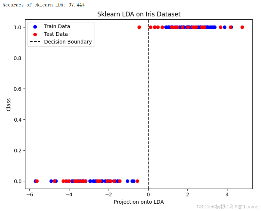
accuracy = accuracy_score(y_test, y_pred)
print(f"Accuracy of sklearn LDA: {accuracy * 100:.2f}%")

# 8. 可视化：将投影到LDA的1维数据
X_train_proj = lda.transform(X_train)
X_test_proj = lda.transform(X_test)

plt.figure(figsize=(8, 6))
plt.scatter(X_train_proj, y_train, color='blue', label='Train Data')
plt.scatter(X_test_proj, y_test, color='red', label='Test Data')
plt.axvline(x=0, color='black', linestyle='--', label='Decision Boundary')
plt.xlabel('Projection onto LDA')
plt.ylabel('Class')
plt.legend()
plt.title('Sklearn LDA on Iris Dataset')
plt.show()

输出结果为：

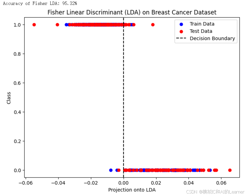
（5）Python代码——示例3——乳腺癌数据集分类——Fisher LDA

import numpy as np
import matplotlib.pyplot as plt
from sklearn import datasets
from sklearn.model_selection import train_test_split
from sklearn.preprocessing import StandardScaler
from sklearn.metrics import accuracy_score

# 1. 加载乳腺癌数据集
cancer = datasets.load_breast_cancer()
X = cancer.data
y = cancer.target

# 2. 标准化特征数据
scaler = StandardScaler()
X = scaler.fit_transform(X)

# 3. 划分训练集和测试集
X_train, X_test, y_train, y_test = train_test_split(X, y, test_size=0.3, random_state=42)

# 4. Fisher线性判别（LDA）的实现

class FisherLDA:
    def __init__(self):
        self.w = None
        self.mu1 = None
        self.mu2 = None
        self.Sw = None
        self.Sb = None
        
    def fit(self, X, y):
        # 类别1和类别2的样本
        X1 = X[y == 0]
        X2 = X[y == 1]
        
        # 计算类别1和类别2的均值
        self.mu1 = np.mean(X1, axis=0)
        self.mu2 = np.mean(X2, axis=0)
        
        # 计算类内散度矩阵 Sw
        self.Sw = np.cov(X1.T) * (len(X1) - 1) + np.cov(X2.T) * (len(X2) - 1)
        
        # 计算类间散度矩阵 Sb
        self.Sb = np.outer(self.mu1 - self.mu2, self.mu1 - self.mu2)
        
        # 计算最佳投影方向 w
        self.w = np.linalg.inv(self.Sw).dot(self.mu1 - self.mu2)
        
    def transform(self, X):
        # 将数据投影到 w 上
        return X.dot(self.w)
    
    def predict(self, X):
        # 将测试数据投影并分类
        X_proj = self.transform(X)
        return np.where(X_proj > 0, 0, 1)  # 投影大于0为恶性（1），否则为良性（0）

# 5. 创建Fisher LDA模型并进行训练
lda = FisherLDA()
lda.fit(X_train, y_train)

# 6. 在测试集上进行预测
y_pred = lda.predict(X_test)

# 7. 计算准确率
accuracy = accuracy_score(y_test, y_pred)
print(f"Accuracy of Fisher LDA: {accuracy * 100:.2f}%")

# 8. 可视化：将投影到LDA的1维数据
X_train_proj = lda.transform(X_train)
X_test_proj = lda.transform(X_test)

plt.figure(figsize=(8, 6))
plt.scatter(X_train_proj, y_train, color='blue', label='Train Data')
plt.scatter(X_test_proj, y_test, color='red', label='Test Data')
plt.axvline(x=0, color='black', linestyle='--', label='Decision Boundary')
plt.xlabel('Projection onto LDA')
plt.ylabel('Class')
plt.legend()
plt.title('Fisher Linear Discriminant (LDA) on Breast Cancer Dataset')
plt.show()

输出结果为：

（6）Python代码——示例3——乳腺癌数据集分类——sklearn中的LDA

import numpy as np
import matplotlib.pyplot as plt
from sklearn import datasets
from sklearn.model_selection import train_test_split
from sklearn.preprocessing import StandardScaler
from sklearn.metrics import accuracy_score
from sklearn.discriminant_analysis import LinearDiscriminantAnalysis

# 1. 加载乳腺癌数据集
cancer = datasets.load_breast_cancer()
X = cancer.data
y = cancer.target

# 2. 标准化特征数据
scaler = StandardScaler()
X = scaler.fit_transform(X)

# 3. 划分训练集和测试集
X_train, X_test, y_train, y_test = train_test_split(X, y, test_size=0.3, random_state=42)

# 4. 使用sklearn中的LDA模型
lda = LinearDiscriminantAnalysis()

# 5. 训练LDA模型
lda.fit(X_train, y_train)

# 6. 在测试集上进行预测
y_pred = lda.predict(X_test)

# 7. 计算准确率
accuracy = accuracy_score(y_test, y_pred)
print(f"Accuracy of sklearn LDA: {accuracy * 100:.2f}%")

# 8. 可视化：将投影到LDA的1维数据
X_train_proj = lda.transform(X_train)
X_test_proj = lda.transform(X_test)

plt.figure(figsize=(8, 6))
plt.scatter(X_train_proj, y_train, color='blue', label='Train Data')
plt.scatter(X_test_proj, y_test, color='red', label='Test Data')
plt.axvline(x=0, color='black', linestyle='--', label='Decision Boundary')
plt.xlabel('Projection onto LDA')
plt.ylabel('Class')
plt.legend()
plt.title('Sklearn LDA on Iris Dataset')
plt.show()

输出结果为：

2、感知机

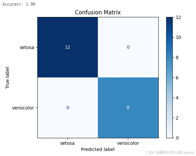
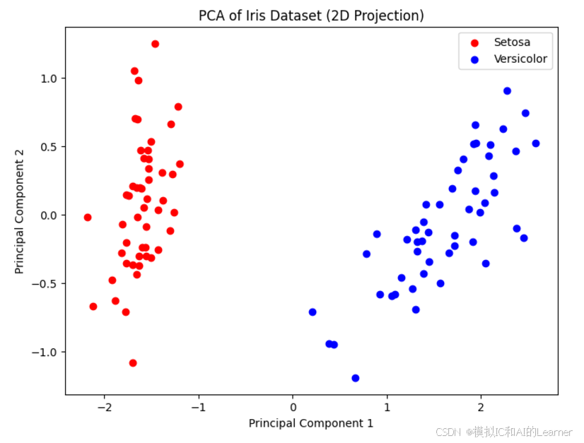
（1）Python代码——示例1——鸢尾花分类

import numpy as np
import pandas as pd
import matplotlib.pyplot as plt
from sklearn.datasets import load_iris
from sklearn.model_selection import train_test_split
from sklearn.linear_model import Perceptron
from sklearn.metrics import accuracy_score, confusion_matrix, ConfusionMatrixDisplay
from sklearn.decomposition import PCA
from mpl_toolkits.mplot3d import Axes3D

# 加载Iris数据集
iris = load_iris()
X = iris.data
y = iris.target
feature_names = iris.feature_names
target_names = iris.target_names

# 选择两个类别进行二分类（可以选择品种0和品种1）
X = X[y != 2]  # 只选择类别0和类别1
y = y[y != 2]  # 只选择类别0和类别1

# 划分训练集和测试集
X_train, X_test, y_train, y_test = train_test_split(X, y, test_size=0.2, random_state=42)

# 初始化并训练感知机模型
model = Perceptron(max_iter=1000, tol=1e-3, random_state=42)
model.fit(X_train, y_train)

# 预测测试集
y_pred = model.predict(X_test)

# 计算准确率
accuracy = accuracy_score(y_test, y_pred)
print(f"Accuracy: {accuracy:.2f}")

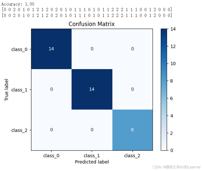
# 计算并显示混淆矩阵
cm = confusion_matrix(y_test, y_pred)
disp = ConfusionMatrixDisplay(confusion_matrix=cm, display_labels=target_names[:2])
disp.plot(cmap='Blues')
plt.title('Confusion Matrix')
plt.show()

# 可视化数据的前两个主成分
pca = PCA(n_components=2)
X_pca = pca.fit_transform(X)

plt.figure(figsize=(8,6))
plt.scatter(X_pca[y == 0, 0], X_pca[y == 0, 1], color='red', label='Setosa')
plt.scatter(X_pca[y == 1, 0], X_pca[y == 1, 1], color='blue', label='Versicolor')
plt.title('PCA of Iris Dataset (2D Projection)')
plt.xlabel('Principal Component 1')
plt.ylabel('Principal Component 2')
plt.legend()
plt.show()

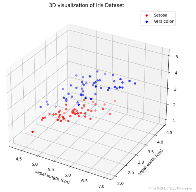
# 3D可视化（选择3个特征）
fig = plt.figure(figsize=(10, 8))
ax = fig.add_subplot(111, projection='3d')
ax.scatter(X[y == 0, 0], X[y == 0, 1], X[y == 0, 2], color='red', label='Setosa')
ax.scatter(X[y == 1, 0], X[y == 1, 1], X[y == 1, 2], color='blue', label='Versicolor')
ax.set_xlabel(feature_names[0])
ax.set_ylabel(feature_names[1])
ax.set_zlabel(feature_names[2])
ax.set_title('3D visualization of Iris Dataset')
ax.legend()
plt.show()

输出结果为：

（2）Python代码——示例2——wine数据集分类

import numpy as np
import matplotlib.pyplot as plt
from sklearn.datasets import load_wine
from sklearn.model_selection import train_test_split
from sklearn.linear_model import Perceptron
from sklearn.metrics import accuracy_score, confusion_matrix, ConfusionMatrixDisplay
from sklearn.decomposition import PCA
from sklearn.preprocessing import StandardScaler

# 加载Wine数据集
wine = load_wine()
X = wine.data
y = wine.target
feature_names = wine.feature_names
target_names = wine.target_names

# 划分训练集和测试集
X_train, X_test, y_train, y_test = train_test_split(X, y, test_size=0.2, random_state=42)

# 标准化数据
scaler = StandardScaler()
X_train = scaler.fit_transform(X_train)
X_test = scaler.transform(X_test)

# 初始化并训练感知机模型
model = Perceptron(max_iter=1000, tol=1e-3, random_state=42)
model.fit(X_train, y_train)

# 预测测试集
y_pred = model.predict(X_test)

# 计算准确率
accuracy = accuracy_score(y_test, y_pred)
print(f"Accuracy: {accuracy:.2f}")
print(y_test)
print(y_pred)

# 计算并显示混淆矩阵
cm = confusion_matrix(y_test, y_pred)
disp = ConfusionMatrixDisplay(confusion_matrix=cm, display_labels=target_names)
disp.plot(cmap='Blues')
plt.title('Confusion Matrix')
plt.show()

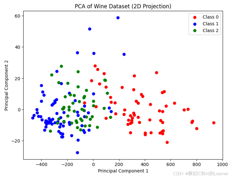
# 可视化数据的前两个主成分
pca = PCA(n_components=2)
X_pca = pca.fit_transform(X)

plt.figure(figsize=(8,6))
plt.scatter(X_pca[y == 0, 0], X_pca[y == 0, 1], color='red', label='Class 0')
plt.scatter(X_pca[y == 1, 0], X_pca[y == 1, 1], color='blue', label='Class 1')
plt.scatter(X_pca[y == 2, 0], X_pca[y == 2, 1], color='green', label='Class 2')
plt.title('PCA of Wine Dataset (2D Projection)')
plt.xlabel('Principal Component 1')
plt.ylabel('Principal Component 2')
plt.legend()
plt.show()

在这次实验中，由于特征比较多，特征之间的量纲差别比较大，如果不进行标准话，精度大大下降，只有0.47。因此数据标准化很重要。

输出结果为：

（3）Python代码——示例3——乳腺癌数据集分类

import numpy as np
import matplotlib.pyplot as plt
from sklearn.datasets import load_breast_cancer
from sklearn.model_selection import train_test_split
from sklearn.linear_model import Perceptron
from sklearn.metrics import accuracy_score, confusion_matrix, ConfusionMatrixDisplay
from sklearn.preprocessing import StandardScaler

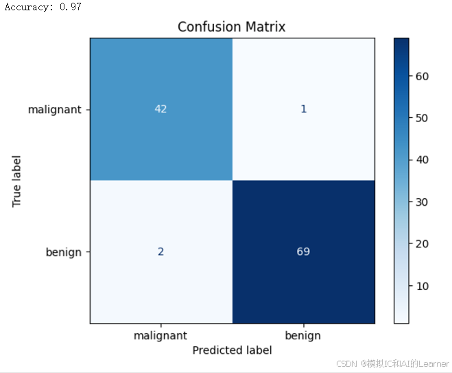
# 加载Breast Cancer Wisconsin数据集
cancer = load_breast_cancer()
X = cancer.data
y = cancer.target
feature_names = cancer.feature_names
target_names = cancer.target_names

# 数据标准化
scaler = StandardScaler()
X_scaled = scaler.fit_transform(X)

# 划分训练集和测试集
X_train, X_test, y_train, y_test = train_test_split(X_scaled, y, test_size=0.2, random_state=42)

# 初始化并训练感知机模型
model = Perceptron(max_iter=1000, tol=1e-3, random_state=42)
model.fit(X_train, y_train)

# 预测测试集
y_pred = model.predict(X_test)

# 计算准确率
accuracy = accuracy_score(y_test, y_pred)
print(f"Accuracy: {accuracy:.2f}")

# 计算并显示混淆矩阵
cm = confusion_matrix(y_test, y_pred)
disp = ConfusionMatrixDisplay(confusion_matrix=cm, display_labels=target_names)
disp.plot(cmap='Blues')
plt.title('Confusion Matrix')
plt.show()

输出结果为：

3、最小平方误差分类器

（1）Python代码——示例1——鸢尾花分类

import numpy as np
import matplotlib.pyplot as plt
from sklearn.datasets import load_iris
from sklearn.model_selection import train_test_split
from sklearn.preprocessing import StandardScaler
from sklearn.linear_model import LinearRegression
from sklearn.metrics import accuracy_score

# 加载Iris数据集
iris = load_iris()
X = iris.data
y = iris.target
target_names = iris.target_names

# 选择类别0和类别1进行二分类（Setosa 和 Versicolor）
X = X[y != 2]  # 只选择类别0和类别1
y = y[y != 2]  # 只选择类别0和类别1

# 划分训练集和测试集
X_train, X_test, y_train, y_test = train_test_split(X, y, test_size=0.2, random_state=42)

# 标准化数据
scaler = StandardScaler()
X_train_scaled = scaler.fit_transform(X_train)
X_test_scaled = scaler.transform(X_test)

# 使用最小平方误差分类器（线性回归）
model = LinearRegression()
model.fit(X_train_scaled, y_train)

# 预测测试集
y_pred = model.predict(X_test_scaled)

# 将预测结果转换为0或1
y_pred_class = (y_pred >= 0.5).astype(int)  # 设定阈值0.5来划分类别

# 计算准确率
accuracy = accuracy_score(y_test, y_pred_class)
print(f"Accuracy: {accuracy:.2f}")

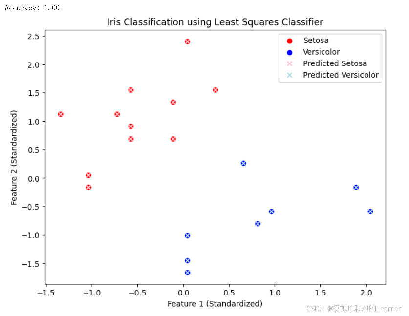
# 可视化结果（只选择前两个特征进行可视化）
plt.figure(figsize=(8, 6))
plt.scatter(X_test_scaled[y_test == 0, 0], X_test_scaled[y_test == 0, 1], color='red', label='Setosa')
plt.scatter(X_test_scaled[y_test == 1, 0], X_test_scaled[y_test == 1, 1], color='blue', label='Versicolor')
plt.scatter(X_test_scaled[y_pred_class == 0, 0], X_test_scaled[y_pred_class == 0, 1], color='pink', marker='x', label='Predicted Setosa')
plt.scatter(X_test_scaled[y_pred_class == 1, 0], X_test_scaled[y_pred_class == 1, 1], color='lightblue', marker='x', label='Predicted Versicolor')
plt.title('Iris Classification using Least Squares Classifier')
plt.xlabel('Feature 1 (Standardized)')
plt.ylabel('Feature 2 (Standardized)')
plt.legend()
plt.show()

输出结果为：

（2）Python代码——示例2——wine数据集分类

import numpy as np
import matplotlib.pyplot as plt
from sklearn.datasets import load_wine
from sklearn.model_selection import train_test_split
from sklearn.preprocessing import StandardScaler
from sklearn.linear_model import LinearRegression
from sklearn.metrics import accuracy_score

# 加载Wine数据集
wine = load_wine()
X = wine.data
y = wine.target
target_names = wine.target_names

# 划分训练集和测试集
X_train, X_test, y_train, y_test = train_test_split(X, y, test_size=0.2, random_state=42)

# 数据标准化
scaler = StandardScaler()
X_train_scaled = scaler.fit_transform(X_train)
X_test_scaled = scaler.transform(X_test)

# 使用最小平方误差分类器（线性回归）进行多分类
def least_squares_classifier(X_train, y_train, X_test):
    # 创建空的预测结果
    y_pred = np.zeros((X_test.shape[0], 3))

    # 训练三个一对多分类器
    for i in range(3):
        # 创建每个类别的训练标签（类别i为1，其他为0）
        y_train_binary = (y_train == i).astype(int)
        
        # 训练最小平方误差分类器（线性回归）
        model = LinearRegression()
        model.fit(X_train, y_train_binary)
        
        # 对测试集进行预测
        y_pred[:, i] = model.predict(X_test)
    
    # 选择最大预测值的类别作为预测结果
    return np.argmax(y_pred, axis=1)

# 训练和预测
y_pred = least_squares_classifier(X_train_scaled, y_train, X_test_scaled)

# 计算准确率
accuracy = accuracy_score(y_test, y_pred)
print(f"Accuracy: {accuracy:.2f}")

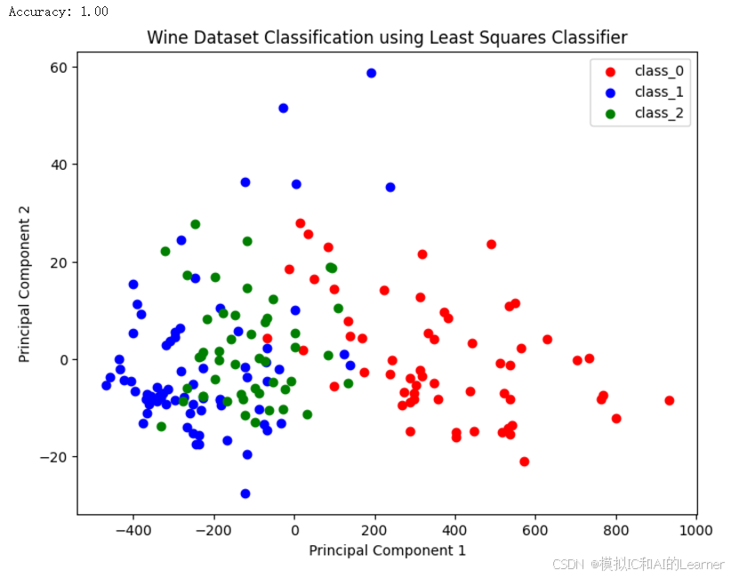
# 可视化结果（使用PCA降维到2D）
from sklearn.decomposition import PCA

# 降维到2D
pca = PCA(n_components=2)
X_pca = pca.fit_transform(X)

# 绘制散点图
plt.figure(figsize=(8, 6))
plt.scatter(X_pca[y == 0, 0], X_pca[y == 0, 1], color='red', label=target_names[0])
plt.scatter(X_pca[y == 1, 0], X_pca[y == 1, 1], color='blue', label=target_names[1])
plt.scatter(X_pca[y == 2, 0], X_pca[y == 2, 1], color='green', label=target_names[2])
plt.title('Wine Dataset Classification using Least Squares Classifier')
plt.xlabel('Principal Component 1')
plt.ylabel('Principal Component 2')
plt.legend()
plt.show()

输出结果为：

（3）Python代码——示例3——乳腺癌数据集分类

import numpy as np
import matplotlib.pyplot as plt
from sklearn.datasets import load_breast_cancer
from sklearn.model_selection import train_test_split
from sklearn.preprocessing import StandardScaler
from sklearn.linear_model import LinearRegression
from sklearn.metrics import accuracy_score

# 加载乳腺癌数据集
cancer = load_breast_cancer()
X = cancer.data
y = cancer.target
target_names = cancer.target_names

# 划分训练集和测试集
X_train, X_test, y_train, y_test = train_test_split(X, y, test_size=0.2, random_state=42)

# 数据标准化
scaler = StandardScaler()
X_train_scaled = scaler.fit_transform(X_train)
X_test_scaled = scaler.transform(X_test)

# 使用最小平方误差分类器（线性回归）
def least_squares_classifier(X_train, y_train, X_test):
    # 创建空的预测结果
    y_pred = np.zeros((X_test.shape[0], 2))  # 对于二分类问题，我们有两个预测值

    # 训练两个一对多分类器
    for i in range(2):
        # 创建每个类别的训练标签（类别i为1，其他为0）
        y_train_binary = (y_train == i).astype(int)
        
        # 训练最小平方误差分类器（线性回归）
        model = LinearRegression()
        model.fit(X_train, y_train_binary)
        
        # 对测试集进行预测
        y_pred[:, i] = model.predict(X_test)
    
    # 选择最大预测值的类别作为预测结果
    return np.argmax(y_pred, axis=1)

# 训练和预测
y_pred = least_squares_classifier(X_train_scaled, y_train, X_test_scaled)

# 计算准确率
accuracy = accuracy_score(y_test, y_pred)
print(f"Accuracy: {accuracy:.2f}")

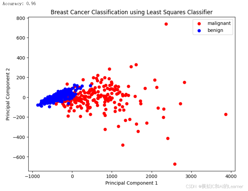
# 可视化结果（如果需要）
# 可以使用PCA进行降维到2D进行简单可视化
from sklearn.decomposition import PCA

# 使用PCA将数据降维到2D
pca = PCA(n_components=2)
X_pca = pca.fit_transform(X)

# 绘制散点图
plt.figure(figsize=(8, 6))
plt.scatter(X_pca[y == 0, 0], X_pca[y == 0, 1], color='red', label=target_names[0])
plt.scatter(X_pca[y == 1, 0], X_pca[y == 1, 1], color='blue', label=target_names[1])
plt.title('Breast Cancer Classification using Least Squares Classifier')
plt.xlabel('Principal Component 1')
plt.ylabel('Principal Component 2')
plt.legend()
plt.show()

输出结果为：

二、广义线性判别函数

通过高阶多项式变换将数据从低维空间映射到高维空间，进而通过线性方法进行分类。这种方式类似于支持向量机（SVM）中的**多项式核（polynomial kernel）**方法，只是这里我们讨论的是一种显式的高阶多项式映射，而不是通过核函数间接映射。

这种做法的关键思想是：即使数据在原始空间中不是线性可分的，我们可以通过高阶多项式映射，将数据投射到一个新的空间，这样在新空间中数据就变得线性可分，从而通过线性判别函数进行分类。

（1）Python代码——示例1——鸢尾花分类

import numpy as np
import pandas as pd
import matplotlib.pyplot as plt
from sklearn.datasets import load_iris
from sklearn.model_selection import train_test_split
from sklearn.preprocessing import StandardScaler
from sklearn.linear_model import LogisticRegression
from sklearn.metrics import classification_report, confusion_matrix
from sklearn.preprocessing import PolynomialFeatures

# 加载鸢尾花数据集
iris = load_iris()
X = iris.data
y = iris.target

# 数据标准化
scaler = StandardScaler()
X_scaled = scaler.fit_transform(X)

# 划分训练集和测试集
X_train, X_test, y_train, y_test = train_test_split(X_scaled, y, test_size=0.3, random_state=42)

# 创建一个多项式特征变换器
poly = PolynomialFeatures(degree=3)  # 3阶多项式变换

# 将训练集和测试集的数据进行多项式变换
X_train_poly = poly.fit_transform(X_train)
X_test_poly = poly.transform(X_test)

# 使用逻辑回归进行分类
clf = LogisticRegression(max_iter=200)
clf.fit(X_train_poly, y_train)

# 预测
y_pred = clf.predict(X_test_poly)

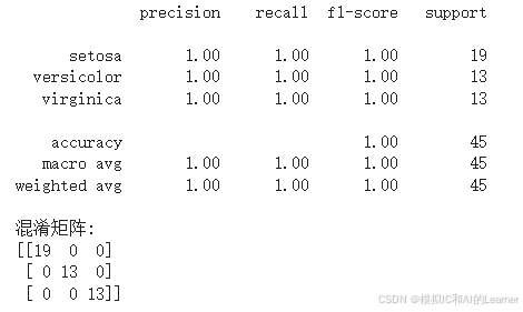
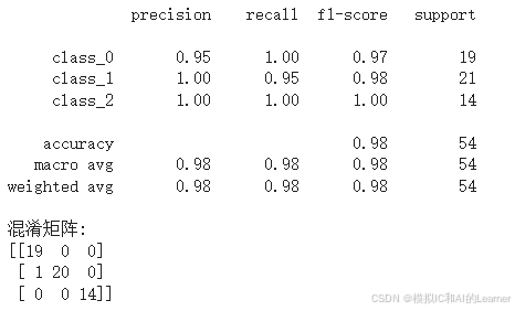
# 打印分类报告
print(classification_report(y_test, y_pred, target_names=iris.target_names))

# 打印混淆矩阵
print("混淆矩阵:")
print(confusion_matrix(y_test, y_pred))

# 可视化
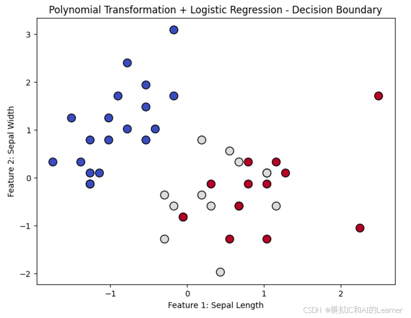
# 为了简化展示，我们只绘制前两个特征的决策边界（即只考虑花萼长度和花萼宽度）

plt.figure(figsize=(8, 6))
plt.scatter(X_test[:, 0], X_test[:, 1], c=y_pred, cmap='coolwarm', marker='o', edgecolors='k', s=100)
plt.title("Polynomial Transformation + Logistic Regression - Decision Boundary")
plt.xlabel("Feature 1: Sepal Length")
plt.ylabel("Feature 2: Sepal Width")
plt.show()

输出结果为：

（2）Python代码——示例2——wine数据集分类

import numpy as np
import pandas as pd
import matplotlib.pyplot as plt
from sklearn.datasets import load_wine
from sklearn.model_selection import train_test_split
from sklearn.preprocessing import StandardScaler
from sklearn.linear_model import LogisticRegression
from sklearn.metrics import classification_report, confusion_matrix
from sklearn.preprocessing import PolynomialFeatures

# 加载 Wine 数据集
wine = load_wine()
X = wine.data
y = wine.target

# 数据标准化
scaler = StandardScaler()
X_scaled = scaler.fit_transform(X)

# 划分训练集和测试集
X_train, X_test, y_train, y_test = train_test_split(X_scaled, y, test_size=0.3, random_state=42)

# 创建一个多项式特征变换器
poly = PolynomialFeatures(degree=3)  # 3阶多项式变换

# 将训练集和测试集的数据进行多项式变换
X_train_poly = poly.fit_transform(X_train)
X_test_poly = poly.transform(X_test)

# 使用逻辑回归进行分类
clf = LogisticRegression(max_iter=200)
clf.fit(X_train_poly, y_train)

# 预测
y_pred = clf.predict(X_test_poly)

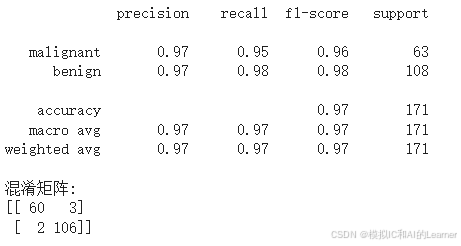
# 打印分类报告
print(classification_report(y_test, y_pred, target_names=wine.target_names))

# 打印混淆矩阵
print("混淆矩阵:")
print(confusion_matrix(y_test, y_pred))

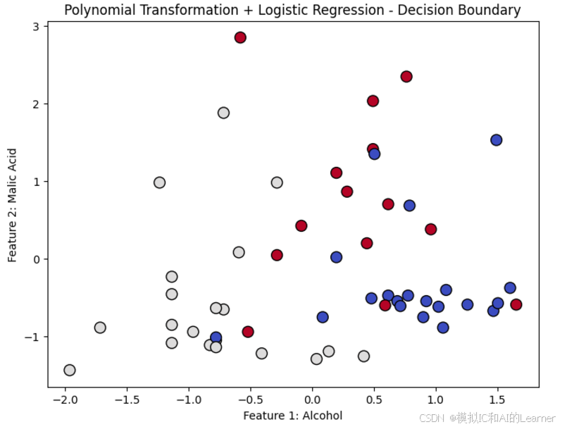
# 可视化（这里只显示前两个特征的决策边界，方便展示）
plt.figure(figsize=(8, 6))
plt.scatter(X_test[:, 0], X_test[:, 1], c=y_pred, cmap='coolwarm', marker='o', edgecolors='k', s=100)
plt.title("Polynomial Transformation + Logistic Regression - Decision Boundary")
plt.xlabel("Feature 1: Alcohol")
plt.ylabel("Feature 2: Malic Acid")
plt.show()

输出结果为：

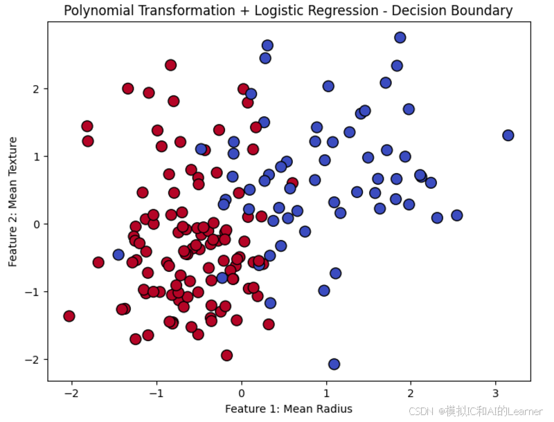
（3）Python代码——示例3——乳腺癌数据集分类

import numpy as np
import pandas as pd
import matplotlib.pyplot as plt
from sklearn.datasets import load_breast_cancer
from sklearn.model_selection import train_test_split
from sklearn.preprocessing import StandardScaler
from sklearn.linear_model import LogisticRegression
from sklearn.metrics import classification_report, confusion_matrix
from sklearn.preprocessing import PolynomialFeatures

# 加载乳腺癌数据集
cancer = load_breast_cancer()
X = cancer.data
y = cancer.target

# 数据标准化
scaler = StandardScaler()
X_scaled = scaler.fit_transform(X)

# 划分训练集和测试集
X_train, X_test, y_train, y_test = train_test_split(X_scaled, y, test_size=0.3, random_state=42)

# 创建一个多项式特征变换器
poly = PolynomialFeatures(degree=3)  # 3阶多项式变换

# 将训练集和测试集的数据进行多项式变换
X_train_poly = poly.fit_transform(X_train)
X_test_poly = poly.transform(X_test)

# 使用逻辑回归进行分类
clf = LogisticRegression(max_iter=200)
clf.fit(X_train_poly, y_train)

# 预测
y_pred = clf.predict(X_test_poly)

# 打印分类报告
print(classification_report(y_test, y_pred, target_names=cancer.target_names))

# 打印混淆矩阵
print("混淆矩阵:")
print(confusion_matrix(y_test, y_pred))

# 可视化（这里只展示前两个特征的决策边界，方便展示）
plt.figure(figsize=(8, 6))
plt.scatter(X_test[:, 0], X_test[:, 1], c=y_pred, cmap='coolwarm', marker='o', edgecolors='k', s=100)
plt.title("Polynomial Transformation + Logistic Regression - Decision Boundary")
plt.xlabel("Feature 1: Mean Radius")
plt.ylabel("Feature 2: Mean Texture")
plt.show()

输出结果为：

（4）Python代码——示例——点击率预估中的因子分解机

!pip install fastFM
import numpy as np
import pandas as pd
from sklearn.model_selection import train_test_split
from sklearn.metrics import mean_squared_error
from fastFM import als
from scipy.sparse import coo_matrix

# 1. 创建假数据集
# 假设我们有三个特征：用户ID (user), 广告ID (ad), 用户所在的设备 (device)
# 目标是预测点击率 (click), click值为0或1，表示是否点击

# 创建样本数据
data = {
    'user': [1, 2, 3, 4, 5, 1, 2, 3, 4, 5],
    'ad': [101, 102, 103, 104, 105, 101, 102, 103, 104, 105],
    'device': [1, 2, 1, 2, 1, 2, 1, 2, 1, 2],
    'click': [0, 1, 0, 1, 0, 1, 0, 1, 0, 1]
}

df = pd.DataFrame(data)

# 2. 数据准备：将数据转换为fastFM所需的格式
# 创建特征映射，以确保每个特征的索引是唯一的
def convert_to_sparse_matrix(df):
    user_map = {user: idx for idx, user in enumerate(df['user'].unique())}
    ad_map = {ad: idx + len(user_map) for idx, ad in enumerate(df['ad'].unique())}
    device_map = {device: idx + len(user_map) + len(ad_map) for idx, device in enumerate(df['device'].unique())}

    rows = []
    cols = []
    data = []
    
    for _, row in df.iterrows():
        # 映射用户、广告、设备到新的索引
        rows.append(row.name)
        cols.append(user_map[row['user']])
        data.append(1)
        
        rows.append(row.name)
        cols.append(ad_map[row['ad']])
        data.append(1)
        
        rows.append(row.name)
        cols.append(device_map[row['device']])
        data.append(1)
    
    X = coo_matrix((data, (rows, cols)), shape=(df.shape[0], len(user_map) + len(ad_map) + len(device_map)))
    y = df['click'].values
    return X, y

X, y = convert_to_sparse_matrix(df)

# 3. 将数据分为训练集和测试集
X_train, X_test, y_train, y_test = train_test_split(X, y, test_size=0.2, random_state=42)

# 4. 使用fastFM库来训练FM模型
# 使用Alternating Least Squares（ALS）算法
fm = als.FMRegression(rank=2, l2_reg_w=0.1, l2_reg_V=0.1, n_iter=100)
fm.fit(X_train, y_train)

# 5. 进行预测并计算模型在测试集上的性能
predictions = fm.predict(X_test)

# 打印预测结果
print("预测结果:", predictions)

# 6. 评估模型性能（使用均方误差作为评估指标）
mse = mean_squared_error(y_test, predictions)
print("均方误差 (MSE):", mse)

这段代码中，数据准备中，将数据转换为fastFM所需的格式，即将数据集转化为稀疏矩阵的形式。

输出结果为：

预测结果: [0.03114698 0.96911975]
均方误差 (MSE): 0.0009618621267152973

三、分段线性判别函数

1、最小距离分类器

（1）介绍

最小距离分类器是一种特殊情况下的分类方法，其假设各类别服从正态分布，且具有相同的协方差矩阵和相等的先验概率。决策规则为，将测试样本归类为距离其最近的类别中心。

假设两类样本的中心分别为 $\mu_1$ 和 $\mu_2$ ，则决策面为两类中心连线的垂直平分面

（2）Python代码——示例——鸢尾花

import numpy as np
from sklearn.datasets import load_iris
from sklearn.model_selection import train_test_split

# 加载鸢尾花数据集
iris = load_iris()
X = iris.data  # 特征数据
y = iris.target  # 标签

# 计算每个类别的均值（中心）
centroids = np.array([X[y == i].mean(axis=0) for i in np.unique(y)])
print(f"每个类别的中心为：",centroids)
# 划分训练集和测试集
X_train, X_test, y_train, y_test = train_test_split(X, y, test_size=0.3, random_state=42)

# 最小距离分类器：计算测试样本到每个类别中心的距离，归类为距离最近的类别
def minimum_distance_classifier(X_train, y_train, X_test):
    # 计算每个类别的均值（中心）
    centroids = np.array([X_train[y_train == i].mean(axis=0) for i in np.unique(y_train)])
    
    # 对于每个测试样本，计算到各个类别中心的距离
    y_pred = []
    for x in X_test:
        # 计算测试样本到每个类别中心的欧几里得距离
        distances = np.linalg.norm(centroids - x, axis=1)
        # 选择距离最小的类别
        y_pred.append(np.argmin(distances))
    
    return np.array(y_pred)

# 使用最小距离分类器进行分类
y_pred = minimum_distance_classifier(X_train, y_train, X_test)

# 输出分类结果
from sklearn.metrics import accuracy_score
accuracy = accuracy_score(y_test, y_pred)
print(f"最小距离分类器在鸢尾花数据集上的分类准确率：{accuracy * 100:.2f}%")

输出结果为：

每个类别的中心为： [[5.006 3.428 1.462 0.246]
 [5.936 2.77  4.26  1.326]
 [6.588 2.974 5.552 2.026]]
最小距离分类器在鸢尾花数据集上的分类准确率：95.56%

2、CART树

CART树（Classification and Regression Trees，分类与回归树）是一种用于分类和回归的决策树算法，由 Breiman et al. 在1986年提出。CART是一种递归的树状结构，能够对数据进行有效的分类和回归预测。其核心思想是通过不断地将数据划分为更纯的子集，最终使得每个叶子节点只包含同一类别的数据（分类任务），或者预测目标值的均值（回归任务）。

（1）Python代码——分类任务示例——鸢尾花数据集

from sklearn.datasets import load_iris
from sklearn.model_selection import train_test_split
from sklearn.tree import DecisionTreeClassifier
from sklearn.metrics import accuracy_score

# 加载鸢尾花数据集
iris = load_iris()
X = iris.data
y = iris.target

# 划分数据集
X_train, X_test, y_train, y_test = train_test_split(X, y, test_size=0.3, random_state=42)

# 初始化CART分类器
clf = DecisionTreeClassifier(criterion='gini', max_depth=3)

# 训练模型
clf.fit(X_train, y_train)

# 预测
y_pred = clf.predict(X_test)

# 输出准确率
accuracy = accuracy_score(y_test, y_pred)
print(f"CART分类器在鸢尾花数据集上的准确率：{accuracy * 100:.2f}%")

输出结果为：

CART分类器在鸢尾花数据集上的准确率：100.00%

（2）Python代码——回归任务示例——加州住房数据集

from sklearn.datasets import fetch_california_housing
from sklearn.model_selection import train_test_split
from sklearn.tree import DecisionTreeRegressor
from sklearn.metrics import mean_squared_error

# 加载加州住房数据集
housing = fetch_california_housing()
X = housing.data
y = housing.target

# 划分数据集
X_train, X_test, y_train, y_test = train_test_split(X, y, test_size=0.3, random_state=42)

# 初始化CART回归器
regressor = DecisionTreeRegressor(max_depth=3)

# 训练模型
regressor.fit(X_train, y_train)

# 预测
y_pred = regressor.predict(X_test)

# 计算均方误差
mse = mean_squared_error(y_test, y_pred)
print(f"CART回归器的均方误差：{mse:.2f}")

输出结果为：