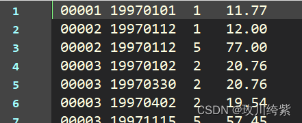
原数据共有69660条数据,有四列,没有列名。
import numpy as np
import pandas as pd
from pandas import DataFrame, Series
import matplotlib.pyplot as plt
第一部分:数据类型处理
- 数据加载
- 字段含义:
- user_id:用户ID
- order_dt:购买日期
- order_product:购买产品的数量
- order_amount:购买金额
- 观察数据
- 查看数据的数据类型
- 数据中是否存储在缺失值
- 将order_dt转换成时间类型
- 查看数据的统计描述
- 计算所有用户购买商品的平均数量
- 计算所有用户购买商品的平均花费
- 在源数据中添加一列表示月份:astype(‘datetime64[M]’)
df = pd.read_csv('./CDNOW_master.txt', header=None, sep='\s+',
names=['user_id', 'order_dt', 'order_product', 'order_amount'])
df.head()
| user_id | order_dt | order_product | order_amount |
|---|
| 0 | 1 | 19970101 | 1 | 11.77 |
|---|
| 1 | 2 | 19970112 | 1 | 12.00 |
|---|
| 2 | 2 | 19970112 | 5 | 77.00 |
|---|
| 3 | 3 | 19970102 | 2 | 20.76 |
|---|
| 4 | 3 | 19970330 | 2 | 20.76 |
|---|
df.info()
<class 'pandas.core.frame.DataFrame'>
RangeIndex: 69659 entries, 0 to 69658
Data columns (total 4 columns):
 #   Column         Non-Null Count  Dtype
---  ------         --------------  -----
 0   user_id        69659 non-null  int64
 1   order_dt       69659 non-null  int64
 2   order_product  69659 non-null  int64
 3   order_amount   69659 non-null  float64
dtypes: float64(1), int64(3)
memory usage: 2.1 MB
df['order_dt'] = pd.to_datetime(df['order_dt'], format='%Y%m%d')
df.info()
<class 'pandas.core.frame.DataFrame'>
RangeIndex: 69659 entries, 0 to 69658
Data columns (total 4 columns):
 #   Column         Non-Null Count  Dtype
---  ------         --------------  -----
 0   user_id        69659 non-null  int64
 1   order_dt       69659 non-null  datetime64[ns]
 2   order_product  69659 non-null  int64
 3   order_amount   69659 non-null  float64
dtypes: datetime64[ns](1), float64(1), int64(2)
memory usage: 2.1 MB
df.describe()
| user_id | order_product | order_amount |
|---|
| count | 69659.000000 | 69659.000000 | 69659.000000 |
|---|
| mean | 11470.854592 | 2.410040 | 35.893648 |
|---|
| std | 6819.904848 | 2.333924 | 36.281942 |
|---|
| min | 1.000000 | 1.000000 | 0.000000 |
|---|
| 25% | 5506.000000 | 1.000000 | 14.490000 |
|---|
| 50% | 11410.000000 | 2.000000 | 25.980000 |
|---|
| 75% | 17273.000000 | 3.000000 | 43.700000 |
|---|
| max | 23570.000000 | 99.000000 | 1286.010000 |
|---|
df['order_dt'].astype('datetime64[M]')
df['month'] = df['order_dt'].astype('datetime64[M]')
df.head()
| user_id | order_dt | order_product | order_amount | month |
|---|
| 0 | 1 | 1997-01-01 | 1 | 11.77 | 1997-01-01 |
|---|
| 1 | 2 | 1997-01-12 | 1 | 12.00 | 1997-01-01 |
|---|
| 2 | 2 | 1997-01-12 | 5 | 77.00 | 1997-01-01 |
|---|
| 3 | 3 | 1997-01-02 | 2 | 20.76 | 1997-01-01 |
|---|
| 4 | 3 | 1997-03-30 | 2 | 20.76 | 1997-03-01 |
|---|
第二部分:按月数据分析
- 用户每月花费的总金额
- 所有用户每月的产品购买量
- 所有用户每月的消费总次数
- 统计每月的消费人数
df.groupby(by='month')['order_amount'].sum()
month
1997-01-01    299060.17
1997-02-01    379590.03
1997-03-01    393155.27
1997-04-01    142824.49
1997-05-01    107933.30
1997-06-01    108395.87
1997-07-01    122078.88
1997-08-01     88367.69
1997-09-01     81948.80
1997-10-01     89780.77
1997-11-01    115448.64
1997-12-01     95577.35
1998-01-01     76756.78
1998-02-01     77096.96
1998-03-01    108970.15
1998-04-01     66231.52
1998-05-01     70989.66
1998-06-01     76109.30
Name: order_amount, dtype: float64
df.groupby(by='month')['order_amount'].sum().plot()
<AxesSubplot:xlabel='month'>
![[外链图片转存失败,源站可能有防盗链机制,建议将图片保存下来直接上传(img-TKd02HMy-1677754166522)(output_9_1.png)]](https://i-blog.csdnimg.cn/blog_migrate/ea2c70f0dce1520bca519a0ffdd8be29.png)
df.groupby(by='month')['order_product'].sum()
month
1997-01-01    19416
1997-02-01    24921
1997-03-01    26159
1997-04-01     9729
1997-05-01     7275
1997-06-01     7301
1997-07-01     8131
1997-08-01     5851
1997-09-01     5729
1997-10-01     6203
1997-11-01     7812
1997-12-01     6418
1998-01-01     5278
1998-02-01     5340
1998-03-01     7431
1998-04-01     4697
1998-05-01     4903
1998-06-01     5287
Name: order_product, dtype: int64
df.groupby(by='month')['user_id'].count()
month
1997-01-01     8928
1997-02-01    11272
1997-03-01    11598
1997-04-01     3781
1997-05-01     2895
1997-06-01     3054
1997-07-01     2942
1997-08-01     2320
1997-09-01     2296
1997-10-01     2562
1997-11-01     2750
1997-12-01     2504
1998-01-01     2032
1998-02-01     2026
1998-03-01     2793
1998-04-01     1878
1998-05-01     1985
1998-06-01     2043
Name: user_id, dtype: int64
df.groupby(by='month')['user_id'].nunique()
month
1997-01-01    7846
1997-02-01    9633
1997-03-01    9524
1997-04-01    2822
1997-05-01    2214
1997-06-01    2339
1997-07-01    2180
1997-08-01    1772
1997-09-01    1739
1997-10-01    1839
1997-11-01    2028
1997-12-01    1864
1998-01-01    1537
1998-02-01    1551
1998-03-01    2060
1998-04-01    1437
1998-05-01    1488
1998-06-01    1506
Name: user_id, dtype: int64
第三部分:用户个体消费数据分析
- 用户消费总金额和消费总次数的统计描述
- 用户消费金额和消费产品数量的散点图
- 各个用户消费总金额的直方分布图(消费金额在1000之内的分布)
- 各个用户消费的总数量的直方分布图(消费商品的数量在100次之内的分布)
df.groupby(by='user_id')['order_amount'].sum()
user_id
1         11.77
2         89.00
3        156.46
4        100.50
5        385.61
          ...
23566     36.00
23567     20.97
23568    121.70
23569     25.74
23570     94.08
Name: order_amount, Length: 23570, dtype: float64
df.groupby(by='user_id')['order_dt'].count()
user_id
1         1
2         2
3         6
4         4
5        11
         ..
23566     1
23567     1
23568     3
23569     1
23570     2
Name: order_dt, Length: 23570, dtype: int64
user_amount_sum = df.groupby(by='user_id')['order_amount'].sum()
user_product_sum = df.groupby(by='user_id')['order_product'].sum()
plt.scatter(user_product_sum, user_amount_sum)
<matplotlib.collections.PathCollection at 0x205b598fcd0>
![[外链图片转存失败,源站可能有防盗链机制,建议将图片保存下来直接上传(img-wb6MtfAD-1677754166523)(output_16_1.png)]](https://i-blog.csdnimg.cn/blog_migrate/e525d7d3d3c2c6afd11334d63db77710.png)
df.groupby(by='user_id').sum().query('order_amount<=1000')['order_amount']
df.groupby(by='user_id').sum().query('order_amount<=1000')['order_amount'].hist()
<AxesSubplot:>
![[外链图片转存失败,源站可能有防盗链机制,建议将图片保存下来直接上传(img-PGmyZDWX-1677754166523)(output_17_1.png)]](https://i-blog.csdnimg.cn/blog_migrate/196dea67532ba02976eba36242874797.png)
df.groupby(by='user_id').sum().query('order_product<=100')['order_product'].hist()
<AxesSubplot:>
![[外链图片转存失败,源站可能有防盗链机制,建议将图片保存下来直接上传(img-JN1dGZ7t-1677754166524)(output_18_1.png)]](https://i-blog.csdnimg.cn/blog_migrate/7cc27d86ac5de7a270af4138ac665ed9.png)
第四部分:用户消费行为分析
- 用户第一次消费的月份分布,和人数统计
- 用户最后一次消费的时间分布,和人数统计
- 新老客户的占比
- 消费一次为新用户
- 消费多次为老用户
- 分析出每一个用户的第一个消费和最后一次消费的时间
- agg([‘func1’,‘func2’]):对分组后的结果进行指定聚合
- 分析出新老客户的消费比例
- 用户分层
- 分析得出每个用户的总购买量和总消费金额and最近一次消费的时间的表格rfm
- RFM模型设计
- R表示客户最近一次交易时间的间隔。
- /np.timedelta64(1,‘D’):去除days
- F表示客户购买商品的总数量,F值越大,表示客户交易越频繁,反之则表示客户交易不够活跃。
- M表示客户交易的金额。M值越大,表示客户价值越高,反之则表示客户价值越低。
- 将R,F,M作用到rfm表中
- 根据价值分层,将用户分为:
- 重要价值客户
- 重要保持客户
- 重要挽留客户
- 重要发展客户
- 一般价值客户
- 一般保持客户
- 一般挽留客户
- 一般发展客户
df.groupby(by='user_id')['month'].min()
user_id
1       1997-01-01
2       1997-01-01
3       1997-01-01
4       1997-01-01
5       1997-01-01
           ...
23566   1997-03-01
23567   1997-03-01
23568   1997-03-01
23569   1997-03-01
23570   1997-03-01
Name: month, Length: 23570, dtype: datetime64[ns]
df.groupby(by='user_id')['month'].min().value_counts()
df.groupby(by='user_id')['month'].min().value_counts().plot()
<AxesSubplot:>
![[外链图片转存失败,源站可能有防盗链机制,建议将图片保存下来直接上传(img-JnxZXA1D-1677754166524)(output_21_1.png)]](https://i-blog.csdnimg.cn/blog_migrate/8d3073ad8aa004d8281a51c46b38fa99.png)
df.groupby(by='user_id')['month'].max().value_counts().plot()
<AxesSubplot:>
![[外链图片转存失败,源站可能有防盗链机制,建议将图片保存下来直接上传(img-gdvlhwba-1677754166525)(output_22_1.png)]](https://i-blog.csdnimg.cn/blog_migrate/684e20388f9c109538e19b295dddb45d.png)
new_old_user_df = df.groupby(by='user_id')['order_dt'].agg(['min', 'max'])
new_old_user_df['min'] == new_old_user_df['max']
(new_old_user_df['min'] == new_old_user_df['max']).value_counts()
True     12054
False    11516
dtype: int64
rfm = df.pivot_table(index='user_id', aggfunc={'order_product': 'sum', 'order_amount': 'sum', 'order_dt': 'max'})
rfm.head()
| order_amount | order_dt | order_product |
|---|
| user_id | | | |
|---|
| 1 | 11.77 | 1997-01-01 | 1 |
|---|
| 2 | 89.00 | 1997-01-12 | 6 |
|---|
| 3 | 156.46 | 1998-05-28 | 16 |
|---|
| 4 | 100.50 | 1997-12-12 | 7 |
|---|
| 5 | 385.61 | 1998-01-03 | 29 |
|---|
max_dt = df['order_dt'].max()
rfm['R'] = (max_dt - rfm['order_dt']) / np.timedelta64(1, 'D')
rfm.head()
| order_amount | order_dt | order_product | R |
|---|
| user_id | | | | |
|---|
| 1 | 11.77 | 1997-01-01 | 1 | 545.0 |
|---|
| 2 | 89.00 | 1997-01-12 | 6 | 534.0 |
|---|
| 3 | 156.46 | 1998-05-28 | 16 | 33.0 |
|---|
| 4 | 100.50 | 1997-12-12 | 7 | 200.0 |
|---|
| 5 | 385.61 | 1998-01-03 | 29 | 178.0 |
|---|
rfm.drop(labels='order_dt', axis=1, inplace=True)
rfm
| order_amount | order_product | R |
|---|
| user_id | | | |
|---|
| 1 | 11.77 | 1 | 545.0 |
|---|
| 2 | 89.00 | 6 | 534.0 |
|---|
| 3 | 156.46 | 16 | 33.0 |
|---|
| 4 | 100.50 | 7 | 200.0 |
|---|
| 5 | 385.61 | 29 | 178.0 |
|---|
| ... | ... | ... | ... |
|---|
| 23566 | 36.00 | 2 | 462.0 |
|---|
| 23567 | 20.97 | 1 | 462.0 |
|---|
| 23568 | 121.70 | 6 | 434.0 |
|---|
| 23569 | 25.74 | 2 | 462.0 |
|---|
| 23570 | 94.08 | 5 | 461.0 |
|---|
23570 rows × 3 columns
rfm.columns = ['M', 'F', 'R']
rfm.head()
| M | F | R |
|---|
| user_id | | | |
|---|
| 1 | 11.77 | 1 | 545.0 |
|---|
| 2 | 89.00 | 6 | 534.0 |
|---|
| 3 | 156.46 | 16 | 33.0 |
|---|
| 4 | 100.50 | 7 | 200.0 |
|---|
| 5 | 385.61 | 29 | 178.0 |
|---|
def rfm_func(x):
level = x.map(lambda x: '1' if x >= 0 else '0')
label = level.R + level.F + level.M
d = {
'111': '重要价值客户',
'011': '重要保持客户',
'101': '重要挽留客户',
'001': '重要发展客户',
'110': '一般价值客户',
'010': '一般保持客户',
'100': '一般挽留客户',
'000': '一般发展客户'
}
result = d[label]
return result
rfm['label'] = rfm.apply(lambda x: x - x.mean()).apply(rfm_func, axis=1)
rfm.head()
| M | F | R | label |
|---|
| user_id | | | | |
|---|
| 1 | 11.77 | 1 | 545.0 | 一般挽留客户 |
|---|
| 2 | 89.00 | 6 | 534.0 | 一般挽留客户 |
|---|
| 3 | 156.46 | 16 | 33.0 | 重要保持客户 |
|---|
| 4 | 100.50 | 7 | 200.0 | 一般发展客户 |
|---|
| 5 | 385.61 | 29 | 178.0 | 重要保持客户 |
|---|
第五部分:用户的生命周期
- 将用户划分为活跃用户和其他用户
- 统计每个用户每个月的消费次数
- 统计每个用户每个月是否消费,消费记录为1否则记录为0
- 知识点:DataFrame的apply和applymap的区别
- applymap:返回df
- 将函数做用于DataFrame中的所有元素(elements)
- apply:返回Series
- apply()将一个函数作用于DataFrame中的每个行或者列
- 将用户按照每一个月份分成:
- unreg:观望用户(前两月没买,第三个月才第一次买,则用户前两个月为观望用户)
- unactive:首月购买后,后序月份没有购买则在没有购买的月份中该用户的为非活跃用户
- new:当前月就进行首次购买的用户在当前月为新用户
- active:连续月份购买的用户在这些月中为活跃用户
- return:购买之后间隔n月再次购买的第一个月份为该月份的回头客
user_month_count_df = df.pivot_table(index='user_id', values='order_dt', aggfunc='count', columns='month').fillna(0)
user_month_count_df.head()
| month | 1997-01-01 | 1997-02-01 | 1997-03-01 | 1997-04-01 | 1997-05-01 | 1997-06-01 | 1997-07-01 | 1997-08-01 | 1997-09-01 | 1997-10-01 | 1997-11-01 | 1997-12-01 | 1998-01-01 | 1998-02-01 | 1998-03-01 | 1998-04-01 | 1998-05-01 | 1998-06-01 |
|---|
| user_id | | | | | | | | | | | | | | | | | | |
|---|
| 1 | 1.0 | 0.0 | 0.0 | 0.0 | 0.0 | 0.0 | 0.0 | 0.0 | 0.0 | 0.0 | 0.0 | 0.0 | 0.0 | 0.0 | 0.0 | 0.0 | 0.0 | 0.0 |
|---|
| 2 | 2.0 | 0.0 | 0.0 | 0.0 | 0.0 | 0.0 | 0.0 | 0.0 | 0.0 | 0.0 | 0.0 | 0.0 | 0.0 | 0.0 | 0.0 | 0.0 | 0.0 | 0.0 |
|---|
| 3 | 1.0 | 0.0 | 1.0 | 1.0 | 0.0 | 0.0 | 0.0 | 0.0 | 0.0 | 0.0 | 2.0 | 0.0 | 0.0 | 0.0 | 0.0 | 0.0 | 1.0 | 0.0 |
|---|
| 4 | 2.0 | 0.0 | 0.0 | 0.0 | 0.0 | 0.0 | 0.0 | 1.0 | 0.0 | 0.0 | 0.0 | 1.0 | 0.0 | 0.0 | 0.0 | 0.0 | 0.0 | 0.0 |
|---|
| 5 | 2.0 | 1.0 | 0.0 | 1.0 | 1.0 | 1.0 | 1.0 | 0.0 | 1.0 | 0.0 | 0.0 | 2.0 | 1.0 | 0.0 | 0.0 | 0.0 | 0.0 | 0.0 |
|---|
df_purchase = user_month_count_df.applymap(lambda x: 1 if x >= 1 else 0)
df_purchase.head()
| month | 1997-01-01 | 1997-02-01 | 1997-03-01 | 1997-04-01 | 1997-05-01 | 1997-06-01 | 1997-07-01 | 1997-08-01 | 1997-09-01 | 1997-10-01 | 1997-11-01 | 1997-12-01 | 1998-01-01 | 1998-02-01 | 1998-03-01 | 1998-04-01 | 1998-05-01 | 1998-06-01 |
|---|
| user_id | | | | | | | | | | | | | | | | | | |
|---|
| 1 | 1 | 0 | 0 | 0 | 0 | 0 | 0 | 0 | 0 | 0 | 0 | 0 | 0 | 0 | 0 | 0 | 0 | 0 |
|---|
| 2 | 1 | 0 | 0 | 0 | 0 | 0 | 0 | 0 | 0 | 0 | 0 | 0 | 0 | 0 | 0 | 0 | 0 | 0 |
|---|
| 3 | 1 | 0 | 1 | 1 | 0 | 0 | 0 | 0 | 0 | 0 | 1 | 0 | 0 | 0 | 0 | 0 | 1 | 0 |
|---|
| 4 | 1 | 0 | 0 | 0 | 0 | 0 | 0 | 1 | 0 | 0 | 0 | 1 | 0 | 0 | 0 | 0 | 0 | 0 |
|---|
| 5 | 1 | 1 | 0 | 1 | 1 | 1 | 1 | 0 | 1 | 0 | 0 | 1 | 1 | 0 | 0 | 0 | 0 | 0 |
|---|
def active_status(data):
status = []
for i in range(18):
if data[i] == 0:
if len(status) > 0:
if status[i-1] == 'unreg':
status.append('unreg')
else:
status.append('unactive')
else:
status.append('unreg')
else:
if len(status) == 0:
status.append('new')
else:
if status[i-1] == 'unactive':
status.append('return')
elif status[i-1] == 'unreg':
status.append('new')
else:
status.append('active')
return status
pivoted_status = df_purchase.apply(active_status,axis = 1)
pivoted_status.head()
user_id
1    [new, unactive, unactive, unactive, unactive, ...
2    [new, unactive, unactive, unactive, unactive, ...
3    [new, unactive, return, active, unactive, unac...
4    [new, unactive, unactive, unactive, unactive, ...
5    [new, active, unactive, return, active, active...
dtype: object
df_purchase_new = DataFrame(data=pivoted_status.values.tolist(),index=df_purchase.index,columns=df_purchase.columns)
df_purchase_new.head()
| month | 1997-01-01 | 1997-02-01 | 1997-03-01 | 1997-04-01 | 1997-05-01 | 1997-06-01 | 1997-07-01 | 1997-08-01 | 1997-09-01 | 1997-10-01 | 1997-11-01 | 1997-12-01 | 1998-01-01 | 1998-02-01 | 1998-03-01 | 1998-04-01 | 1998-05-01 | 1998-06-01 |
|---|
| user_id | | | | | | | | | | | | | | | | | | |
|---|
| 1 | new | unactive | unactive | unactive | unactive | unactive | unactive | unactive | unactive | unactive | unactive | unactive | unactive | unactive | unactive | unactive | unactive | unactive |
|---|
| 2 | new | unactive | unactive | unactive | unactive | unactive | unactive | unactive | unactive | unactive | unactive | unactive | unactive | unactive | unactive | unactive | unactive | unactive |
|---|
| 3 | new | unactive | return | active | unactive | unactive | unactive | unactive | unactive | unactive | return | unactive | unactive | unactive | unactive | unactive | return | unactive |
|---|
| 4 | new | unactive | unactive | unactive | unactive | unactive | unactive | return | unactive | unactive | unactive | return | unactive | unactive | unactive | unactive | unactive | unactive |
|---|
| 5 | new | active | unactive | return | active | active | active | unactive | return | unactive | unactive | return | active | unactive | unactive | unactive | unactive | unactive |
|---|
- 每月【不同活跃】用户的计数
- purchase_status_ct = df_purchase_new.apply(lambda x : pd.value_counts(x)).fillna(0)
- 转置进行最终结果的查看
purchase_status_ct = df_purchase_new.apply(lambda x : pd.value_counts(x)).fillna(0)
purchase_status_ct
| month | 1997-01-01 | 1997-02-01 | 1997-03-01 | 1997-04-01 | 1997-05-01 | 1997-06-01 | 1997-07-01 | 1997-08-01 | 1997-09-01 | 1997-10-01 | 1997-11-01 | 1997-12-01 | 1998-01-01 | 1998-02-01 | 1998-03-01 | 1998-04-01 | 1998-05-01 | 1998-06-01 |
|---|
| active | 0.0 | 1157.0 | 1681.0 | 1773.0 | 852.0 | 747.0 | 746.0 | 604.0 | 528.0 | 532.0 | 624.0 | 632.0 | 512.0 | 472.0 | 571.0 | 518.0 | 459.0 | 446.0 |
|---|
| new | 7846.0 | 8476.0 | 7248.0 | 0.0 | 0.0 | 0.0 | 0.0 | 0.0 | 0.0 | 0.0 | 0.0 | 0.0 | 0.0 | 0.0 | 0.0 | 0.0 | 0.0 | 0.0 |
|---|
| return | 0.0 | 0.0 | 595.0 | 1049.0 | 1362.0 | 1592.0 | 1434.0 | 1168.0 | 1211.0 | 1307.0 | 1404.0 | 1232.0 | 1025.0 | 1079.0 | 1489.0 | 919.0 | 1029.0 | 1060.0 |
|---|
| unactive | 0.0 | 6689.0 | 14046.0 | 20748.0 | 21356.0 | 21231.0 | 21390.0 | 21798.0 | 21831.0 | 21731.0 | 21542.0 | 21706.0 | 22033.0 | 22019.0 | 21510.0 | 22133.0 | 22082.0 | 22064.0 |
|---|
| unreg | 15724.0 | 7248.0 | 0.0 | 0.0 | 0.0 | 0.0 | 0.0 | 0.0 | 0.0 | 0.0 | 0.0 | 0.0 | 0.0 | 0.0 | 0.0 | 0.0 | 0.0 | 0.0 |
|---|
purchase_status_ct.T
| active | new | return | unactive | unreg |
|---|
| month | | | | | |
|---|
| 1997-01-01 | 0.0 | 7846.0 | 0.0 | 0.0 | 15724.0 |
|---|
| 1997-02-01 | 1157.0 | 8476.0 | 0.0 | 6689.0 | 7248.0 |
|---|
| 1997-03-01 | 1681.0 | 7248.0 | 595.0 | 14046.0 | 0.0 |
|---|
| 1997-04-01 | 1773.0 | 0.0 | 1049.0 | 20748.0 | 0.0 |
|---|
| 1997-05-01 | 852.0 | 0.0 | 1362.0 | 21356.0 | 0.0 |
|---|
| 1997-06-01 | 747.0 | 0.0 | 1592.0 | 21231.0 | 0.0 |
|---|
| 1997-07-01 | 746.0 | 0.0 | 1434.0 | 21390.0 | 0.0 |
|---|
| 1997-08-01 | 604.0 | 0.0 | 1168.0 | 21798.0 | 0.0 |
|---|
| 1997-09-01 | 528.0 | 0.0 | 1211.0 | 21831.0 | 0.0 |
|---|
| 1997-10-01 | 532.0 | 0.0 | 1307.0 | 21731.0 | 0.0 |
|---|
| 1997-11-01 | 624.0 | 0.0 | 1404.0 | 21542.0 | 0.0 |
|---|
| 1997-12-01 | 632.0 | 0.0 | 1232.0 | 21706.0 | 0.0 |
|---|
| 1998-01-01 | 512.0 | 0.0 | 1025.0 | 22033.0 | 0.0 |
|---|
| 1998-02-01 | 472.0 | 0.0 | 1079.0 | 22019.0 | 0.0 |
|---|
| 1998-03-01 | 571.0 | 0.0 | 1489.0 | 21510.0 | 0.0 |
|---|
| 1998-04-01 | 518.0 | 0.0 | 919.0 | 22133.0 | 0.0 |
|---|
| 1998-05-01 | 459.0 | 0.0 | 1029.0 | 22082.0 | 0.0 |
|---|
| 1998-06-01 | 446.0 | 0.0 | 1060.0 | 22064.0 | 0.0 |
|---|
参考视频:【2022年张晓波亲授【数据分析自学课程】它来了!必备的Excel/SQL/Tableau/Python/数据黑话数据分析启蒙免费课程教程】 https://www.bilibili.com/video/BV1Bi4y1m7k7/?p=29&share_source=copy_web&vd_source=1170c577d779798202386e1f343fe38b


 该文展示了使用Python的Pandas库对电商数据进行预处理,包括数据类型转换、缺失值检查、统计分析等。然后,分析了用户按月的消费总金额、产品购买量和消费次数,揭示了各月消费趋势。接着,对单个用户进行了消费总金额、消费总次数的统计描述,并绘制了散点图。最后,通过RFM模型分析了用户的价值层级,以及用户生命周期的不同阶段,如新用户、活跃用户、回头客等。


 700
700

 被折叠的 条评论
为什么被折叠?
被折叠的 条评论
为什么被折叠?
 到【灌水乐园】发言


