Python + 模拟退火

原创已于 2025-08-09 18:46:27 修改 · 1k 阅读

CC 4.0 BY-SA版权

文章标签：

于 2025-07-15 10:39:47 首次发布

模拟退火（Simulated Annealing，SA）是一种用于全局优化问题的随机化算法，受到物理中“退火”过程的启发。退火是金属从高温慢慢冷却到低温的过程，其中金属分子从混乱的状态逐渐变得有序。模拟退火利用类似的策略来找到一个优化问题的最优解。

一、工作原理

模拟退火的核心思想是通过模拟金属退火的过程，在搜索空间中逐渐寻找最优解。具体步骤如下：

1.初始状态和温度设定：从一个随机解开始，设定一个较高的初始温度（类似于物理过程中的温度）。
2.生成邻域解：通过小的随机变化生成当前解的邻域解（即稍微改变当前解的某些参数）。
3.接受准则：

如果邻域解比当前解更好（即目标函数值更小或更大，取决于优化方向），则接受该邻域解。

4.降温过程：逐步降低温度（“冷却”过程）。温度的下降通常是指数型的，即每次降温的幅度逐渐减小。温度的降低意味着接受更差解的概率变小，从而收敛到一个最优解。
5.终止条件：当温度降到某个较低值，或达到预定的最大迭代次数时，停止搜索，最终得到一个解。

# 1、设定一个初始温度T(这个温度很高)
# 2、每次循环都退火一次
# 3、然后降低T的温度，我们通过让和 T 一个降温系数 dT（一个接近1的小数）相乘，达到慢慢降低温度的效果，直接接近于0（（我们用eps来代表一个接近0的数）只要 T < eps 就可以退出循环）

T = 2000    # 初始温度
dT = 0.99   # 降温系数 delta T
eps = 1e-14 # 温度下限阈值

while T > eps:  # 循环条件：当温度高于阈值时继续退火
    # 这里写每次的退火操作

    T = T * dT  # 温度按系数下降

二、模拟退火的优点

全局搜索能力强：模拟退火通过接受较差解避免了陷入局部最优解，增加了找到全局最优解的可能性。
简单易实现：算法的结构简单，且不需要复杂的数学推导，易于实现。

三、模拟退火的缺点

计算时间较长：尤其是在需要多次降温或温度下降较慢时，算法可能需要较长的时间才能找到较好的解。
调参困难：温度的初始值、降温速率等参数的选择可能对结果有较大影响，往往需要多次实验进行调整。

四、应用领域

组合优化问题：如旅行商问题、图着色问题、生产调度问题等。
机器学习与数据挖掘：比如特征选择、模型参数调优等。
物理和化学领域：如蛋白质折叠问题、材料设计等。

五、代码演示部分

列题1：找到这个函数的最小值

1、python代码

from __future__ import division
import numpy as np
import math


# 定义目标函数（待优化的函数）
def aimFunction(x):
    y = x ** 3 - 60 * x ** 2 - 4 * x + 6
    return y


# 模拟退火算法参数初始化
T = 1000  # 初始温度
Tmin = 10  # 终止温度（温度下限）
x = np.random.uniform(low=0, high=100)  # 随机初始化自变量x
k = 50  # 内循环次数（每个温度下的迭代次数）
y = 0  # 目标函数值初始化
t = 0  # 迭代计数

# 模拟退火主循环：当温度大于等于终止温度时继续迭代
while T >= Tmin:
    for i in range(k):
        # 计算当前解的目标函数值
        y = aimFunction(x)

        # 在当前解的邻域内生成一个新解（扰动）
        # 邻域大小与温度T成正比，随着温度降低，搜索范围逐渐缩小
        xNew = x + np.random.uniform(low=-0.055, high=0.055) * T

        # 检查新解是否在定义域[0, 100]内
        if (0 <= xNew and xNew <= 100):
            yNew = aimFunction(xNew)

            # 如果新解更优（目标函数值更小），则接受新解
            if yNew - y < 0:
                x = xNew
            else:
                # 否则，依据Metropolis准则以一定概率接受较差解
                # 这个概率随着温度降低而减小
                p = math.exp(-(yNew - y) / T) # 注意负号
                r = np.random.uniform(low=0, high=1)
                if r < p:
                    x = xNew

    # 温度更新（降温）
    t += 1
    print(f"迭代次数: {t}, 当前温度: {T:.2f}")
    T = 1000 / (1 + t)  # 降温函数，随迭代次数增加温度逐渐降低 可以自己定义一个dT降温系数: T = T * dT

# 输出最优解及其对应的目标函数值
print(f"最优解 x = {x:.6f}, 目标函数值 y = {aimFunction(x):.6f}")

2、控制台展示：

E:\python\python.exe D:\compiler\python\建模\模拟退火test\1.py
迭代次数: 1, 当前温度: 1000.00
迭代次数: 2, 当前温度: 500.00
迭代次数: 3, 当前温度: 333.33
迭代次数: 4, 当前温度: 250.00
迭代次数: 5, 当前温度: 200.00
迭代次数: 6, 当前温度: 166.67
迭代次数: 7, 当前温度: 142.86
迭代次数: 8, 当前温度: 125.00
迭代次数: 9, 当前温度: 111.11
迭代次数: 10, 当前温度: 100.00
迭代次数: 11, 当前温度: 90.91
迭代次数: 12, 当前温度: 83.33
迭代次数: 13, 当前温度: 76.92
迭代次数: 14, 当前温度: 71.43
迭代次数: 15, 当前温度: 66.67
迭代次数: 16, 当前温度: 62.50
迭代次数: 17, 当前温度: 58.82
迭代次数: 18, 当前温度: 55.56
迭代次数: 19, 当前温度: 52.63
迭代次数: 20, 当前温度: 50.00
迭代次数: 21, 当前温度: 47.62
迭代次数: 22, 当前温度: 45.45
迭代次数: 23, 当前温度: 43.48
迭代次数: 24, 当前温度: 41.67
迭代次数: 25, 当前温度: 40.00
迭代次数: 26, 当前温度: 38.46
迭代次数: 27, 当前温度: 37.04
迭代次数: 28, 当前温度: 35.71
迭代次数: 29, 当前温度: 34.48
迭代次数: 30, 当前温度: 33.33
迭代次数: 31, 当前温度: 32.26
迭代次数: 32, 当前温度: 31.25
迭代次数: 33, 当前温度: 30.30
迭代次数: 34, 当前温度: 29.41
迭代次数: 35, 当前温度: 28.57
迭代次数: 36, 当前温度: 27.78
迭代次数: 37, 当前温度: 27.03
迭代次数: 38, 当前温度: 26.32
迭代次数: 39, 当前温度: 25.64
迭代次数: 40, 当前温度: 25.00
迭代次数: 41, 当前温度: 24.39
迭代次数: 42, 当前温度: 23.81
迭代次数: 43, 当前温度: 23.26
迭代次数: 44, 当前温度: 22.73
迭代次数: 45, 当前温度: 22.22
迭代次数: 46, 当前温度: 21.74
迭代次数: 47, 当前温度: 21.28
迭代次数: 48, 当前温度: 20.83
迭代次数: 49, 当前温度: 20.41
迭代次数: 50, 当前温度: 20.00
迭代次数: 51, 当前温度: 19.61
迭代次数: 52, 当前温度: 19.23
迭代次数: 53, 当前温度: 18.87
迭代次数: 54, 当前温度: 18.52
迭代次数: 55, 当前温度: 18.18
迭代次数: 56, 当前温度: 17.86
迭代次数: 57, 当前温度: 17.54
迭代次数: 58, 当前温度: 17.24
迭代次数: 59, 当前温度: 16.95
迭代次数: 60, 当前温度: 16.67
迭代次数: 61, 当前温度: 16.39
迭代次数: 62, 当前温度: 16.13
迭代次数: 63, 当前温度: 15.87
迭代次数: 64, 当前温度: 15.62
迭代次数: 65, 当前温度: 15.38
迭代次数: 66, 当前温度: 15.15
迭代次数: 67, 当前温度: 14.93
迭代次数: 68, 当前温度: 14.71
迭代次数: 69, 当前温度: 14.49
迭代次数: 70, 当前温度: 14.29
迭代次数: 71, 当前温度: 14.08
迭代次数: 72, 当前温度: 13.89
迭代次数: 73, 当前温度: 13.70
迭代次数: 74, 当前温度: 13.51
迭代次数: 75, 当前温度: 13.33
迭代次数: 76, 当前温度: 13.16
迭代次数: 77, 当前温度: 12.99
迭代次数: 78, 当前温度: 12.82
迭代次数: 79, 当前温度: 12.66
迭代次数: 80, 当前温度: 12.50
迭代次数: 81, 当前温度: 12.35
迭代次数: 82, 当前温度: 12.20
迭代次数: 83, 当前温度: 12.05
迭代次数: 84, 当前温度: 11.90
迭代次数: 85, 当前温度: 11.76
迭代次数: 86, 当前温度: 11.63
迭代次数: 87, 当前温度: 11.49
迭代次数: 88, 当前温度: 11.36
迭代次数: 89, 当前温度: 11.24
迭代次数: 90, 当前温度: 11.11
迭代次数: 91, 当前温度: 10.99
迭代次数: 92, 当前温度: 10.87
迭代次数: 93, 当前温度: 10.75
迭代次数: 94, 当前温度: 10.64
迭代次数: 95, 当前温度: 10.53
迭代次数: 96, 当前温度: 10.42
迭代次数: 97, 当前温度: 10.31
迭代次数: 98, 当前温度: 10.20
迭代次数: 99, 当前温度: 10.10
迭代次数: 100, 当前温度: 10.00
最优解 x = 40.215724, 目标函数值 y = -32152.060650

进程已结束，退出代码为 0

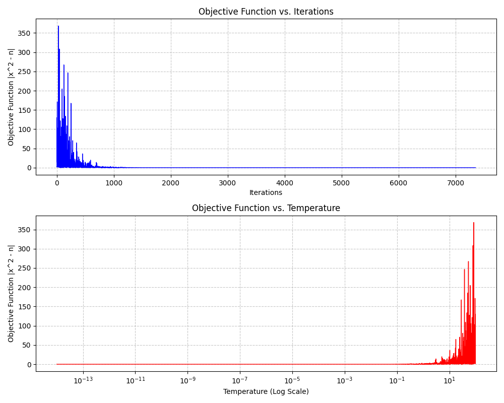
列题2：找到 n 的算数平方根

1、python代码

from __future__ import division
import numpy as np
import math
import matplotlib.pyplot as plt


# 获取用户输入
n = float(input("Enter a positive number: "))

# 目标函数：|x^2 - n|
def aimFunction(x):
    return math.fabs(x * x - n)

# 模拟退火参数
T = max(100, n)  # 初始温度
Tmin = 1e-14     # 终止温度
dT = 0.995       # 降温系数
x = np.random.uniform(low=0, high=np.sqrt(n)*2)  # 初始解
k = 30           # 内循环次数
history = []     # 记录迭代过程

# 主循环
while T >= Tmin:
    for i in range(k):
        y = aimFunction(x)
        # 生成新解（扰动）
        xNew = x + np.random.uniform(-1, 1) * T * 0.1
        if xNew >= 0:  # 确保非负
            yNew = aimFunction(xNew)
            # 接受准则
            if yNew < y or np.random.random() < math.exp(-(yNew - y)/T):
                x = xNew
    history.append((T, x, aimFunction(x)))
    T *= dT  # 降温
    # 打印进度
    if len(history) % 100 == 0:
        print(f"Iteration: {len(history)}, Temperature: {T:.6f}, Current Best: {x:.6f}")

# 输出结果
print(f"\nInput Value: {n}")
print(f"Calculated Square Root: {x:.10f}")
print(f"Actual Square Root: {math.sqrt(n):.10f}")
print(f"Absolute Error: {abs(x - math.sqrt(n)):.10f}")

# 提取绘图数据
iterations = range(1, len(history)+1)
temperatures = [h[0] for h in history]
objective_values = [h[2] for h in history]

# 绘图（使用英文标签，避免中文）
plt.figure(figsize=(10, 8))

# 子图1：目标函数随迭代次数变化
plt.subplot(2, 1, 1)  # 创建2行1列的子图布局，选择第1个子图（上方）
plt.plot(iterations, objective_values, 'b-', linewidth=1)  # 绘制蓝色实线
plt.xlabel('Iterations')  # x轴标签：迭代次数
plt.ylabel('Objective Function |x^2 - n|')  # y轴标签：目标函数值
plt.title('Objective Function vs. Iterations')  # 子图标题
plt.grid(True, linestyle='--', alpha=0.7)  # 添加虚线网格（透明度70%）

# 子图2：目标函数随温度变化
plt.subplot(2, 1, 2)  # 选择第2个子图（下方）
plt.plot(temperatures, objective_values, 'r-', linewidth=1)  # 绘制红色实线
plt.xscale('log')  # 设置x轴为对数尺度（因为温度指数下降）
plt.xlabel('Temperature (Log Scale)')  # x轴标签：温度（对数尺度）
plt.ylabel('Objective Function |x^2 - n|')  # y轴标签：目标函数值
plt.title('Objective Function vs. Temperature')  # 子图标题
plt.grid(True, linestyle='--', alpha=0.7)  # 添加虚线网格

plt.tight_layout()  # 自动调整子图参数，避免标签重叠
plt.show()  # 显示图形

2、控制台展示：

E:\python\python.exe D:\compiler\python\建模\模拟退火test\2.py
Enter a positive number: 2
Iteration: 100, Temperature: 60.577044, Current Best: 1.384569
Iteration: 200, Temperature: 36.695782, Current Best: 6.986883
Iteration: 300, Temperature: 22.229220, Current Best: 1.302009
Iteration: 400, Temperature: 13.465804, Current Best: 3.457651
Iteration: 500, Temperature: 8.157186, Current Best: 1.348156
Iteration: 600, Temperature: 4.941382, Current Best: 1.481375
Iteration: 700, Temperature: 2.993343, Current Best: 1.213146
Iteration: 800, Temperature: 1.813279, Current Best: 1.414416
Iteration: 900, Temperature: 1.098431, Current Best: 1.683188
Iteration: 1000, Temperature: 0.665397, Current Best: 1.431369
Iteration: 1100, Temperature: 0.403078, Current Best: 1.260856
Iteration: 1200, Temperature: 0.244173, Current Best: 1.497106
Iteration: 1300, Temperature: 0.147913, Current Best: 1.270650
Iteration: 1400, Temperature: 0.089601, Current Best: 1.335943
Iteration: 1500, Temperature: 0.054278, Current Best: 1.426471
Iteration: 1600, Temperature: 0.032880, Current Best: 1.429626
Iteration: 1700, Temperature: 0.019918, Current Best: 1.416934
Iteration: 1800, Temperature: 0.012066, Current Best: 1.413867
Iteration: 1900, Temperature: 0.007309, Current Best: 1.417952
Iteration: 2000, Temperature: 0.004428, Current Best: 1.414231
Iteration: 2100, Temperature: 0.002682, Current Best: 1.414696
Iteration: 2200, Temperature: 0.001625, Current Best: 1.414136
Iteration: 2300, Temperature: 0.000984, Current Best: 1.414561
Iteration: 2400, Temperature: 0.000596, Current Best: 1.414203
Iteration: 2500, Temperature: 0.000361, Current Best: 1.414287
Iteration: 2600, Temperature: 0.000219, Current Best: 1.414233
Iteration: 2700, Temperature: 0.000133, Current Best: 1.414250
Iteration: 2800, Temperature: 0.000080, Current Best: 1.414256
Iteration: 2900, Temperature: 0.000049, Current Best: 1.414253
Iteration: 3000, Temperature: 0.000029, Current Best: 1.414216
Iteration: 3100, Temperature: 0.000018, Current Best: 1.414218
Iteration: 3200, Temperature: 0.000011, Current Best: 1.414227
Iteration: 3300, Temperature: 0.000007, Current Best: 1.414215
Iteration: 3400, Temperature: 0.000004, Current Best: 1.414216
Iteration: 3500, Temperature: 0.000002, Current Best: 1.414212
Iteration: 3600, Temperature: 0.000001, Current Best: 1.414214
Iteration: 3700, Temperature: 0.000001, Current Best: 1.414215
Iteration: 3800, Temperature: 0.000001, Current Best: 1.414214
Iteration: 3900, Temperature: 0.000000, Current Best: 1.414213
Iteration: 4000, Temperature: 0.000000, Current Best: 1.414214
Iteration: 4100, Temperature: 0.000000, Current Best: 1.414214
Iteration: 4200, Temperature: 0.000000, Current Best: 1.414214
Iteration: 4300, Temperature: 0.000000, Current Best: 1.414214
Iteration: 4400, Temperature: 0.000000, Current Best: 1.414214
Iteration: 4500, Temperature: 0.000000, Current Best: 1.414214
Iteration: 4600, Temperature: 0.000000, Current Best: 1.414214
Iteration: 4700, Temperature: 0.000000, Current Best: 1.414214
Iteration: 4800, Temperature: 0.000000, Current Best: 1.414214
Iteration: 4900, Temperature: 0.000000, Current Best: 1.414214
Iteration: 5000, Temperature: 0.000000, Current Best: 1.414214
Iteration: 5100, Temperature: 0.000000, Current Best: 1.414214
Iteration: 5200, Temperature: 0.000000, Current Best: 1.414214
Iteration: 5300, Temperature: 0.000000, Current Best: 1.414214
Iteration: 5400, Temperature: 0.000000, Current Best: 1.414214
Iteration: 5500, Temperature: 0.000000, Current Best: 1.414214
Iteration: 5600, Temperature: 0.000000, Current Best: 1.414214
Iteration: 5700, Temperature: 0.000000, Current Best: 1.414214
Iteration: 5800, Temperature: 0.000000, Current Best: 1.414214
Iteration: 5900, Temperature: 0.000000, Current Best: 1.414214
Iteration: 6000, Temperature: 0.000000, Current Best: 1.414214
Iteration: 6100, Temperature: 0.000000, Current Best: 1.414214
Iteration: 6200, Temperature: 0.000000, Current Best: 1.414214
Iteration: 6300, Temperature: 0.000000, Current Best: 1.414214
Iteration: 6400, Temperature: 0.000000, Current Best: 1.414214
Iteration: 6500, Temperature: 0.000000, Current Best: 1.414214
Iteration: 6600, Temperature: 0.000000, Current Best: 1.414214
Iteration: 6700, Temperature: 0.000000, Current Best: 1.414214
Iteration: 6800, Temperature: 0.000000, Current Best: 1.414214
Iteration: 6900, Temperature: 0.000000, Current Best: 1.414214
Iteration: 7000, Temperature: 0.000000, Current Best: 1.414214
Iteration: 7100, Temperature: 0.000000, Current Best: 1.414214
Iteration: 7200, Temperature: 0.000000, Current Best: 1.414214
Iteration: 7300, Temperature: 0.000000, Current Best: 1.414214

Input Value: 2.0
Calculated Square Root: 1.4142135624
Actual Square Root: 1.4142135624
Absolute Error: 0.0000000000

3、生成图展示：

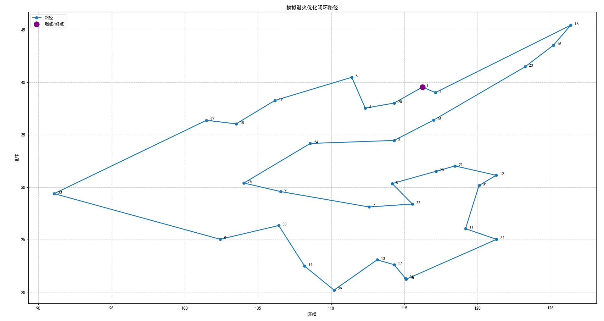
例题3：已知全国34个省会城市（包括直辖市、自治区首府和港澳台）的经纬度坐标（第一个为北京）；现在需要从北京出发，到所有城市视察，要求每个城市只能到达一次，并最终回到北京。求视察路线方案，使得总路径最短。（TSP旅行商问题）

1、excel数据

2、python代码

import numpy as np
import matplotlib.pyplot as plt
import pandas as pd
import math

# 设置中文显示
plt.rcParams["font.family"] = ["SimHei", "Microsoft YaHei"]
plt.rcParams["axes.unicode_minus"] = False  # 解决负号显示问题


# 定义距离计算函数（球面距离）
def distance(lat1, lon1, lat2, lon2, radius=6371):
    """计算球面上两点之间的距离（单位：km）"""
    lon1, lat1, lon2, lat2 = map(math.radians, [lon1, lat1, lon2, lat2])
    dlon = lon2 - lon1
    dlat = lat2 - lat1
    a = math.sin(dlat / 2) ** 2 + math.cos(lat1) * math.cos(lat2) * math.sin(dlon / 2) ** 2
    c = 2 * math.atan2(math.sqrt(a), math.sqrt(1 - a))
    return radius * c


def generate_initial_solution(d, num_cities=34, start_city=0, end_city=0):
    """生成旅行商问题的初始解（确保起点终点正确，支持闭环）"""
    # 确保起点和终点有效
    if start_city < 0 or start_city >= num_cities:
        start_city = 0
    if end_city < 0 or end_city >= num_cities:
        end_city = start_city  # 默认为闭环（起点=终点）

    # 生成中间城市的随机排列（排除起点，因为终点和起点相同）
    middle_cities = np.random.permutation(np.setdiff1d(np.arange(num_cities), [start_city]))
    # 构建完整路径：起点 → 中间城市 → 终点（闭环）
    path = [start_city] + list(middle_cities) + [end_city]

    # 计算路径总长度（包含最后一段回到起点的距离）
    total_length = 0
    for i in range(len(path) - 1):
        total_length += d[path[i]][path[i + 1]]

    return path, total_length


def simulated_annealing_tsp(d, city, initial_path, initial_length, start_city=0, end_city=0,
                            e=1e-30, alpha=0.999, T=100, markov=100):
    """模拟退火算法求解旅行商问题（支持起点终点相同的闭环路径）"""
    path = initial_path.copy()
    current_length = initial_length
    best_path = path.copy()
    best_length = current_length

    accept = 0
    rand_accept = 0
    refuse = 0
    num_cities = len(city)

    # 固定起点和终点（支持闭环）
    if path[0] != start_city:
        path.insert(0, start_city)
    if path[-1] != end_city:
        path.append(end_city)

    while T > e:
        for _ in range(markov):
            # 只在中间城市进行交换（避开起点和终点）
            if len(path) < 4:  # 至少需要2个中间城市才能交换
                continue
            # 选择范围：1到len(path)-2（确保起点0和终点-1不被修改）
            u, v = np.sort(np.random.randint(1, len(path) - 1, 2))

            # 计算目标函数增量（只计算受影响的边）
            df = d[path[u - 1], path[v]] + d[path[u], path[v + 1]] - \
                 d[path[u - 1], path[u]] - d[path[v], path[v + 1]]

            # 接受准则
            if df < 0:
                # 直接接受更优解
                path[u:v + 1] = path[u:v + 1][::-1]  # 逆序u到v的城市
                current_length += df
                accept += 1

                # 更新全局最优
                if current_length < best_length:
                    best_length = current_length
                    best_path = path.copy()

            elif np.exp(-df / T) >= np.random.rand():
                # 以概率接受更差解
                path[u:v + 1] = path[u:v + 1][::-1]
                current_length += df
                rand_accept += 1

                # 更新全局最优
                if current_length < best_length:
                    best_length = current_length
                    best_path = path.copy()
            else:
                # 拒绝新解
                refuse += 1

        # 降温
        T *= alpha

    # 若为闭环路径，确保最后一段距离正确（中间城市到终点/起点）
    if start_city == end_city and len(best_path) >= 2:
        last_middle = best_path[-2]
        # 重新计算最后一段距离（覆盖可能的错误累积）
        final_segment = distance(
            city[last_middle, 1], city[last_middle, 0],
            city[end_city, 1], city[end_city, 0]
        )
        # 修正总长度：减去旧的最后一段距离，加上正确的距离
        best_length = best_length - d[best_path[-2]][best_path[-1]] + final_segment
        best_path[-1] = end_city  # 确保终点正确

    return best_path, best_length, {'accept': accept, 'rand_accept': rand_accept, 'refuse': refuse}


def plot_tsp_path(city, path, start_city=0, end_city=0, title="TSP闭环路径"):
    """可视化TSP闭环路径，突出显示起点/终点"""
    plt.figure(figsize=(12, 10))

    # 路径有效性检查
    valid_indices = set(range(len(city)))
    invalid = [p for p in path if p not in valid_indices]
    if invalid:
        print(f"警告：路径中存在无效索引 {invalid}，已自动过滤")
        path = [p for p in path if p in valid_indices]

    # 确保路径包含起点和终点（闭环）
    if not path:
        path = [start_city, end_city]
    if path[0] != start_city:
        path.insert(0, start_city)
    if path[-1] != end_city:
        path.append(end_city)

    # 转换为numpy数组
    path_np = np.array(path)

    # 绘制完整路径（闭环）
    plt.plot(city[path_np, 0], city[path_np, 1], 'o-',
             color='#1f77b4', linewidth=2, markersize=6,
             label='路径')

    # 突出显示起点/终点（闭环时是同一个点）
    plt.scatter(city[start_city, 0], city[start_city, 1],
                color='purple', s=150, zorder=5, label='起点/终点')

    # 标记城市编号
    for i in range(len(city)):
        plt.text(city[i, 0], city[i, 1], f"  {i + 1}", fontsize=9)

    plt.xlabel('东经')
    plt.ylabel('北纬')
    plt.title(title)
    plt.grid(True, linestyle='--', alpha=0.7)
    plt.legend()
    plt.tight_layout()
    plt.show()


# 验证闭环路径各段距离
def print_path_segments(city, path, d):
    total = 0
    print("\n路径各段距离：")
    for i in range(len(path) - 1):
        from_city = path[i]
        to_city = path[i + 1]
        dist = d[from_city][to_city]
        total += dist
        print(f"城市 {from_city + 1} → 城市 {to_city + 1}: {dist:.2f} km")
    print(f"总距离（闭环）: {total:.2f} km")


def main():
    # 配置起点和终点（闭环：起点=终点=0）
    START_CITY = 0
    END_CITY = 0  # 与起点相同，形成闭环

    # 读取城市数据
    try:
        data = pd.read_excel('cities.xlsx', header=0, usecols=[1, 2])
        city = data.values
        n = city.shape[0]
        if n == 0:
            raise ValueError("城市数据为空，请检查Excel文件")
        print(f"成功读取 {n} 个城市数据")
    except Exception as e:
        print(f"读取城市数据失败：{e}")
        # 生成模拟数据（如果读取失败）
        np.random.seed(42)
        n = 34
        city = np.random.rand(n, 2) * 100  # 模拟经纬度数据
        print(f"使用模拟数据，生成 {n} 个城市")

    # 初始化距离矩阵
    d = np.zeros((n, n))
    for i in range(n):
        for j in range(n):
            d[i, j] = distance(city[i, 1], city[i, 0], city[j, 1], city[j, 0])

    # 生成初始解（闭环路径）
    initial_path, initial_length = generate_initial_solution(
        d, num_cities=n, start_city=START_CITY, end_city=END_CITY
    )
    print(f"初始路径长度: {initial_length:.2f} km")
    print(f"初始路径: {initial_path[:5]}...{initial_path[-5:]}")  # 只显示部分路径

    # 使用模拟退火算法优化路径
    best_path, best_length, stats = simulated_annealing_tsp(
        d, city, initial_path, initial_length,
        start_city=START_CITY, end_city=END_CITY,
        e=1e-30, alpha=0.999, T=3000, markov=100
    )

    # 输出结果统计
    print(f"优化后路径: {best_path[:5]}...{best_path[-5:]}")
    print(f"优化后路径长度: {best_length:.2f} km")
    print(f"优化比例: {(1 - best_length / initial_length) * 100:.2f}%")
    print(f"直接接受新解次数: {stats['accept']}")
    print(f"接受更差的随机解次数: {stats['rand_accept']}")
    print(f"不接受随机解次数: {stats['refuse']}")
    # 在main函数中调用（优化路径之后）
    print_path_segments(city, best_path, d)
    # 可视化结果（闭环路径）
    plot_tsp_path(city, best_path, START_CITY, END_CITY, title="模拟退火优化闭环路径")


if __name__ == "__main__":
    main()

3、控制台输出

E:\python\python.exe D:\compiler\python\建模\启发式算法\模拟退火test\1test\main.py
成功读取 34 个城市数据
初始路径长度: 46110.71 km
初始路径: [0, np.int64(8), np.int64(27), np.int64(15), np.int64(33)]...[np.int64(9), np.int64(17), np.int64(12), np.int64(14), 0]
优化后路径: [0, np.int64(1), np.int64(15), np.int64(14), np.int64(22)]...[np.int64(18), np.int64(5), np.int64(3), np.int64(19), 0]
优化后路径长度: 13878.74 km
优化比例: 69.90%
直接接受新解次数: 134934
接受更差的随机解次数: 214322
不接受随机解次数: 7355344

路径各段距离：
城市 1 → 城市 2: 95.96 km
城市 2 → 城市 16: 1041.98 km
城市 16 → 城市 15: 230.75 km
城市 15 → 城市 23: 278.83 km
城市 23 → 城市 25: 781.40 km
城市 25 → 城市 3: 326.13 km
城市 3 → 城市 24: 527.17 km
城市 24 → 城市 26: 597.41 km
城市 26 → 城市 9: 257.04 km
城市 9 → 城市 7: 611.37 km
城市 7 → 城市 22: 291.57 km
城市 22 → 城市 8: 254.74 km
城市 8 → 城市 28: 314.30 km
城市 28 → 城市 21: 134.48 km
城市 21 → 城市 12: 283.96 km
城市 12 → 城市 31: 156.21 km
城市 31 → 城市 11: 465.83 km
城市 11 → 城市 32: 241.04 km
城市 32 → 城市 18: 760.01 km
城市 18 → 城市 34: 12.27 km
城市 34 → 城市 17: 163.95 km
城市 17 → 城市 13: 129.40 km
城市 13 → 城市 29: 441.43 km
城市 29 → 城市 14: 328.03 km
城市 14 → 城市 30: 466.13 km
城市 30 → 城市 5: 426.42 km
城市 5 → 城市 33: 1220.44 km
城市 33 → 城市 27: 1242.50 km
城市 27 → 城市 10: 186.01 km
城市 10 → 城市 19: 341.49 km
城市 19 → 城市 6: 513.71 km
城市 6 → 城市 4: 336.43 km
城市 4 → 城市 20: 181.17 km
城市 20 → 城市 1: 239.19 km
总距离（闭环）: 13878.74 km