重学SurfaceFlinger之Layer显示区域bounds计算剖析

原创于 2025-12-19 23:19:00 发布 · 280 阅读

8 ·

CC 4.0 BY-SA版权

文章标签：

#智能手机 #android #安卓framework开发 #车载开发 #SurfaceFlinger #sf #Layer

surfaceflinger 专栏收录该内容

58 篇文章

订阅专栏

背景

有学员在学习SurfaceFlinger相关课程时候，就问过经常在SurfaceFlinger中看到某个Layer有自己的显示bounds区域，而且还有好几个和bounds相关的变量，也不太清楚这个bounds计算是怎么计算出来的，对这块的理解比较疑惑，希望马哥可以搞个文章解释一下。
在这里插入图片描述

核心代码部分：

相关变量


    // Cached properties computed from drawing state
    // Effective transform taking into account parent transforms and any parent scaling, which is
    // a transform from the current layer coordinate space to display(screen) coordinate space.
    ui::Transform mEffectiveTransform;

    // Bounds of the layer before any transformation is applied and before it has been cropped
    // by its parents.
    FloatRect mSourceBounds;

    // Bounds of the layer in layer space. This is the mSourceBounds cropped by its layer crop and
    // its parent bounds.
    FloatRect mBounds;

    // Layer bounds in screen space.
    FloatRect mScreenBounds;

这里其实因为也注释很详细，这里简单中文解释如下：
mSourceBounds：图像原本有多大

mBounds：图像能显示多少，因为可能会经过被裁剪crop遮挡，或者parent区域限制

mEffectiveTransform：图像摆在哪里、怎么摆，是否有偏移放大等操作

mScreenBounds：屏幕上看到图像在哪、有多大

原始内容 (mSourceBounds)
    ↓ 裁剪1：自身裁剪crop
    ↓ 裁剪2：父边界约束（不能超出父层）
裁剪后内容 (mBounds)
    ↓ 应用变换矩阵 (mEffectiveTransform)
屏幕上的最终位置 (mScreenBounds)

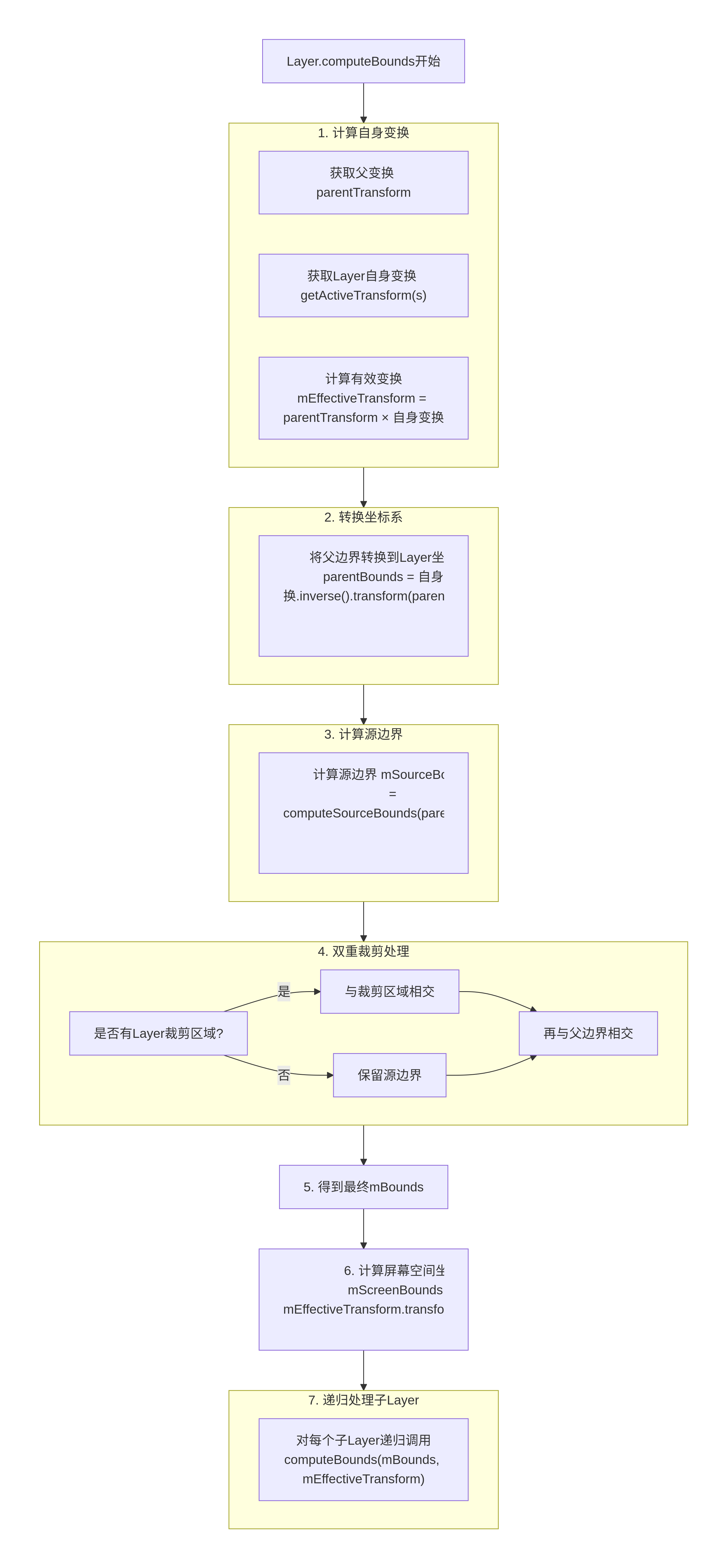
使用这些变量场景主要是在computeBounds方法进行Layer的bounds计算时候，所以只有深入剖析computeBounds才可以更加深入理解这些变量。


void Layer::computeBounds(FloatRect parentBounds, ui::Transform parentTransform,
                          float parentShadowRadius) {
    const State& s(getDrawingState());

//当前获取Layer的transform，由parentTransform和DrawingState共同相差决定，父亲transform会影响子Layer
    // Calculate effective layer transform
    mEffectiveTransform = parentTransform * getActiveTransform(s);

    // Transform parent bounds to layer space
    parentBounds = getActiveTransform(s).inverse().transform(parentBounds);
//计算当前Layer sourcebound可以简单认为是自身buffer区域，但是没有buffer那就用parentBounds
    // Calculate source bounds
    mSourceBounds = computeSourceBounds(parentBounds);

    // Calculate bounds by croping diplay frame with layer crop and parent bounds
    FloatRect bounds = mSourceBounds;
    //获取是否有裁剪
    const Rect layerCrop = getCrop(s);
    if (!layerCrop.isEmpty()) {
    //如果设置了crop裁剪bound那么会与sourceBounds进行相交处理
        bounds = mSourceBounds.intersect(layerCrop.toFloatRect());
    }
    
    //上面计算得出的bounds还需要与parent的Bounds进行相交处理，故不可以超过父Layer的bounds大小
    bounds = bounds.intersect(parentBounds);
//赋值给Layer的成员变量mBounds
    mBounds = bounds;
    //mBounds只是说显示Layer的bounds大小范围，但是显示的坐标是最后确定靠以下的transform确定
    mScreenBounds = mEffectiveTransform.transform(mBounds);

//省略部分
    //接下来需要调用Layer的孩子分别调用computeBounds进行bounds计算
    for (const sp<Layer>& child : mDrawingChildren) {
    //可以看到这里直接传递的是mEffectiveTransform作为parentTransform
        child->computeBounds(mBounds, mEffectiveTransform, childShadowRadius);
    }

//省略部分
}

上面注释已经写的比较详细，这里对一些方法也进行额外补充解释。

看看这里的computeSourceBounds方法

FloatRect Layer::computeSourceBounds(const FloatRect& parentBounds) const {
//这里可以看到对于非buffer的layer是直接使用父亲的，比如task
    if (mBufferInfo.mBuffer == nullptr) {
        return parentBounds;
    }

    return getBufferSize(getDrawingState()).toFloatRect();
}

可以得出当前Layer只有有buffer的SourceBounds才会自己的buffer的bounds，不然都是parentBounds。
在这里插入图片描述看完这些代码，大家可能已经比较熟悉，但是还希望有一个案例可以更加形象的说明就好了。

案例举例

一、简单案例设定

假设：

屏幕坐标系：
原点在左上角，x向右，y向下。

父Layer（比如是一个全屏的窗口）：

父Layer的变换：没有变换，即单位矩阵。

父Layer的边界：整个屏幕，假设为 (0, 0, 1000, 1000)。

子Layer（当前Layer）：

子Layer自身变换：没有缩放和旋转，只有平移，比如向右下角平移(200, 300)。

子Layer的Buffer大小（内容大小）：(0, 0, 400, 300)。

子Layer没有设置裁剪区域（layerCrop为空）。

二、计算过程
步骤1：计算有效变换矩阵

父变换parentTransform：单位矩阵
子层自身变换getActiveTransform(s)：平移(200,300)
mEffectiveTransform = 父变换 × 子层自身变换 = 平移(200,300)

步骤2：将父边界转换到子层局部坐标系

子层自身变换的逆矩阵：平移(-200, -300)
父边界parentBounds: (0,0,1000,1000)
转换后：平移(-200,-300).transform( (0,0,1000,1000) ) = (-200,-300,800,700)
注意：这里我们假设变换只影响顶点，实际上变换矩阵会作用于每个点，但平移变换只是将矩形偏移。

步骤3：计算源边界（mSourceBounds）

调用computeSourceBounds，传入转换后的父边界(-200,-300,800,700)
由于子层有Buffer，大小为(0,0,400,300)，所以mSourceBounds = (0,0,400,300)

步骤4：第一层裁剪（Layer自身Crop）

layerCrop为空，所以跳过，bounds = mSourceBounds = (0,0,400,300)

步骤5：第二层裁剪（父边界约束）

bounds与转换后的父边界相交：
(0,0,400,300) 与 (-200,-300,800,700) 相交 = (0,0,400,300)
因为子层的源边界完全在转换后的父边界内，所以不变。

步骤6：得到最终mBounds

mBounds = (0,0,400,300)

步骤7：计算屏幕边界（mScreenBounds）

mScreenBounds = mEffectiveTransform.transform(mBounds)
= 平移(200,300).transform( (0,0,400,300) )
= (200,300,600,600)

三、结果解释

子Layer在自己的局部坐标系中，它的可显示区域是(0,0,400,300)，即整个Buffer。

在屏幕坐标系中，由于子Layer平移了(200,300)，所以它的显示区域变为(200,300,600,600)。

四、考虑有裁剪的情况

假设其他条件不变，子Layer设置了一个裁剪区域：

layerCrop = (50,50,350,250) // 注意：这个裁剪区域是在子层局部坐标系中

那么步骤4变为：

bounds = mSourceBounds.intersect(layerCrop.toFloatRect())
= (0,0,400,300) 与 (50,50,350,250) 相交
= (50,50,350,250)

步骤5：

bounds与转换后的父边界相交：
(50,50,350,250) 与 (-200,-300,800,700) 相交 = (50,50,350,250)

步骤6：

mBounds = (50,50,350,250)

步骤7：

mScreenBounds = 平移(200,300).transform( (50,50,350,250) )
= (250,350,550,550)

这样，子Layer在屏幕上只显示了(250,350)到(550,550)的区域，即被裁剪后的部分。
五、考虑子Layer超出父边界的情况

假设子Layer的平移量更大，比如平移(900,900)，其他条件不变（无裁剪）。

步骤2：

转换后的父边界：平移(-900,-900).transform( (0,0,1000,1000) ) = (-900,-900,100,100)

步骤3：不变，mSourceBounds = (0,0,400,300)

步骤4：不变，bounds = (0,0,400,300)

步骤5：与转换后的父边界相交

(0,0,400,300) 与 (-900,-900,100,100) 相交 = (0,0,100,100)

注意：因为转换后的父边界在子层坐标系中只有(-900,-900)到(100,100)的区域，所以相交后只有(0,0,100,100)部分可见。

步骤6：
mBounds = (0,0,100,100)

步骤7：

mScreenBounds = 平移(900,900).transform( (0,0,100,100) )
              = (900,900,1000,1000)

这样，子Layer只有左上角(0,0)到(100,100)的部分被显示在屏幕的(900,900)到(1000,1000)区域，其余部分被父边界裁剪掉了。
六、总结

通过这个简单案例，我们可以看到computeBounds的核心思想：

通过逆变换将父边界转换到子层坐标系，以便在同一个坐标系中进行裁剪。

子层的内容（源边界）先与自身的裁剪区域相交，再与父边界相交，得到最终在子层坐标系中的边界（mBounds）。

然后通过有效变换将mBounds变换到屏幕坐标系，得到屏幕上的实际显示区域（mScreenBounds）。

这样的设计保证了每一层都只显示在父层允许的范围内，并且可以方便地应用自身的裁剪。