


 光学相干断层扫描(OCT)是一种无创的视网膜评估技术,利用激光光扫描视网膜,能详细显示视网膜各层。OCT对于涉及黄斑部的疾病特别有用,可帮助精确定位视网膜损伤,辅助诊断和治疗进程评估,如老年黄斑变性和糖尿病黄斑水肿。此外,OCT还能用于评估手术需求,如Epiretinal Membranes和Macular Holes的情况。
此文有助于医学图象处理的初学者对OCT图像有一个简单的认识。
1. What is Optical Coherence Tomography?
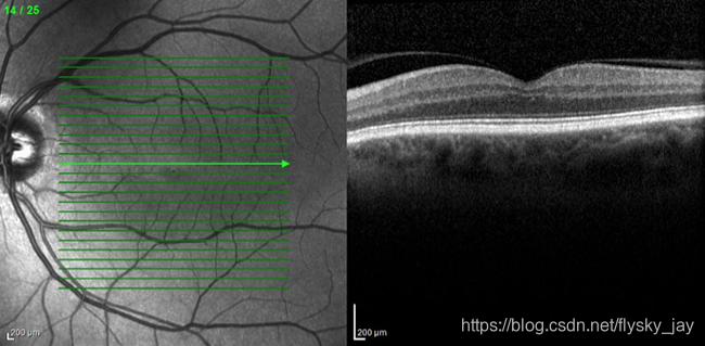
Optical Coherence Tomography (OCT) is a non-invasive imaging technique used to evaluate the retina. The image is acquired using laser light to scan the retina and results in an image that shows the retinal layers in great detail. When looking at an OCT scan we see it as if the retina were cut in half and seen from the side. This allows all the layers to be visualized all the way back to the wall of the eye, the sclera.
How are they helpful?
OCT’s can be useful in any condition that affects the macula, the center of the retina. While retinal damage is seen on clinical exam, being able to localize the damage to a particular layer of the retina can help further characterize the process. OCT’s can also be used to help determine how a condition is responding to treatment or progressing such as with Age Related Macular Degeneration and Diabetic Macular Edema. Lesions can be measured with the scans and in patients with Epiretinal Membranes and Macular Holes that can help determine if surgery is necessary and the expected response.
OCT血流成像图像采集
OCT血流成像结构图示


 1755
1755

 被折叠的 条评论
为什么被折叠?
被折叠的 条评论
为什么被折叠?
 到【灌水乐园】发言


