


Reinforcement Learning Control of a Nonlinear Chemical Reactor
I. INTRODUCTION
The design of control systems for chemical reactors is typically based on simplified and linear models that do not adequately represent the actual behavior of industrial processes. The industrial reactor is characterized by highly nonlinear behavior and multivariable dynamics, which makes traditional control strategies less effective. Therefore, there is a need to evaluate new control methodologies capable of handling these complexities.
In recent years, control schemes based on Reinforcement Learning (RL) have gained attention due to their ability to learn optimal control policies through interaction with the environment without requiring an explicit mathematical model of the system. RL-based controllers can adapt to time-varying and nonlinear processes, making them suitable for complex industrial applications such as continuous stirred-tank reactors (CSTR).
This study focuses on the application of a Model-Free Reinforcement Learning (MFRL) algorithm called Q-Learning to control a nonlinear chemical reactor known as the Klatt-Engell reactor. First, the mathematical model of the plant will be presented to build the nonlinear state equations. Then, a controller will be designed based on two sub-controllers using the Q-Learning algorithm, selecting characteristics of states, actions, rewards, and other parameters of RL. Finally, simulations of the control system will be performed for reference functions, stepped variables, and sinusoidal inputs.
Keywords—Reinforcement learning, learning, controller, temperature control, state, action, reward, Q-learning, reactor, Klatt, Engell, nonlinear, temperature, component
II. MATHEMATICAL MODEL OF THE KLATT-ENGELL REACTOR
The reactor model described by Klatt and Engell [5], [6] is used. This model shows interesting nonlinear behavior depending on the setpoints and is useful for comparison with other models since it presents some favorable properties. The high complexity of the reactor can be used for comparison and avoids including distorting effects that would result from model reduction. Furthermore, the Klatt-Engell reactor is interesting from an industrial application viewpoint since it represents a whole class of CSTRs with jacket cooling.
The reactor is fed with a solution of a reactant $ A $ at a certain concentration $ C_{A,in} $ and the chemical reaction going on inside the reactor follows the van de Vusse scheme, where the main reaction $ A \rightarrow B $ is accompanied by a side reaction $ 2A \rightarrow D $, and it follows up a reaction $ B \rightarrow C $, both yielding undesired by-products $ D $ and $ C $ [7]. The list of variables and parameters of the Klatt-Engell reactor is described in Table I [7], [8].
TABLE I
Variables and Parameters of the Plant
| Symbol | Description |
|---|---|
| $ C_A $ | Concentration of component A inside the reactor (mol/L) |
| $ C_B $ | Concentration of component B inside the reactor (mol/L) |
| $ T $ | Temperature inside the reactor (K) |
| $ T_j $ | Jacket temperature (K) |
| $ k_1 $ | Activation energy divided by gas constant for reaction 1 (K) |
| $ k_2 $ | Activation energy divided by gas constant for reaction 2 (K) |
| $ k_3 $ | Activation energy divided by gas constant for reaction 3 (K) |
| $ E_1 $ | Activation energy for reaction 1 (kJ/mol) |
| $ E_2 $ | Activation energy for reaction 2 (kJ/mol) |
| $ E_3 $ | Activation energy for reaction 3 (kJ/mol) |
| $ V $ | Volume inside the reactor (L) |
| $ V_j $ | Volume of the jacket (L) |
| $ \rho $ | Density of the medium inside the reactor (kg/L) |
| $ \rho_j $ | Density of the medium inside the jacket (kg/L) |
| $ C_p $ | Heat capacity of the medium inside the reactor (kJ/kg·K) |
| $ C_{p,j} $ | Heat capacity of the medium inside the jacket (kJ/kg·K) |
| $ A_j $ | Surface area of the jacket (m²) |
| $ U $ | Heat transfer coefficient (kJ/s·m²·K) |
| $ m_j $ | Jacket mass (kg) |
| $ C_{p,m} $ | Heat capacity of the jacket material (kJ/kg·K) |
| $ F $ | Feed flow rate (L/s) |
| $ Q_j $ | Heat flow applied to the jacket (kJ/s) |
| $ T_{in} $ | Inlet temperature (K) |
| $ C_{A,in} $ | Inlet concentration of component A (mol/L) |
A. Mathematical Model Equations of the Klatt-Engell Reactor
As with any other systems, chemical systems must conform to the laws of mass and energy conservation. The Klatt-Engell reactor model comprises two material balances for the concentration of the reactant $ A $ and product $ B $, as well as energy balances for the reactor and the cooling jacket with temperatures $ T $ and $ T_j $ respectively [7]. The system of ordinary differential equations of the plant is as follows:
$$
\frac{dC_A}{dt} = \frac{F}{V}(C_{A,in} - C_A) - k_1 \exp\left(-\frac{E_1}{RT}\right)C_A - k_2 \exp\left(-\frac{E_2}{RT}\right)C_A^2 \tag{1}
$$
$$
\frac{dC_B}{dt} = -\frac{F}{V}C_B + k_1 \exp\left(-\frac{E_1}{RT}\right)C_A - k_3 \exp\left(-\frac{E_3}{RT}\right)C_B \tag{2}
$$
$$
\frac{dT}{dt} = \frac{F}{V}(T_{in} - T) + \frac{-\Delta H_1 k_1 \exp\left(-\frac{E_1}{RT}\right)C_A - \Delta H_2 k_2 \exp\left(-\frac{E_2}{RT}\right)C_A^2 - \Delta H_3 k_3 \exp\left(-\frac{E_3}{RT}\right)C_B}{\rho C_p} + \frac{U A_j (T_j - T)}{\rho C_p V} \tag{3}
$$
$$
\frac{dT_j}{dt} = \frac{1}{m_j C_{p,m}} \left(Q_j - U A_j (T_j - T)\right) \tag{4}
$$
The parameter values are summarized in Table II [7], [8].
TABLE II
Nominal Parameter Values of the Plant
| Parameter | Value | Unit |
|---|---|---|
| $ V $ | 1.1 | L |
| $ V_j $ | 0.5 | L |
| $ \rho $ | 0.934 | kg/L |
| $ \rho_j $ | 0.95 | kg/L |
| $ C_p $ | 3.01 | kJ/kg·K |
| $ C_{p,j} $ | 4.184 | kJ/kg·K |
| $ A_j $ | 0.215 | m² |
| $ U $ | 67.2 | kJ/s·m²·K |
| $ m_j $ | 0.5 | kg |
| $ C_{p,m} $ | 0.4 | kJ/kg·K |
| $ F $ | 0.0033 | L/s |
| $ Q_j $ | Variable | kJ/s |
| $ T_{in} $ | 104 | K |
| $ C_{A,in} $ | 5.1 | mol/L |
| $ k_1 $ | 18.97 | 1/s |
| $ k_2 $ | 27.10 | 1/s |
| $ k_3 $ | 2.71 | 1/s |
| $ E_1 $ | 9758.3 | K |
| $ E_2 $ | 9758.3 | K |
| $ E_3 $ | 8560 | K |
| $ \Delta H_1 $ | -4.2 | kJ/mol |
| $ \Delta H_2 $ | -11.2 | kJ/mol |
| $ \Delta H_3 $ | -4.2 | kJ/mol |
The input flow rate $ F $ (scaled by the volume of the reactor $ V $) and the heat flow $ Q_j $ serve as manipulated inputs:
$$
u_1 = \frac{F}{V}, \quad u_2 = Q_j \tag{5}
$$
Both inputs are subject to constraints in terms of lower and upper bounds:
$$
0 \leq u_1 \leq 0.01 \tag{6}
$$
$$
0 \leq u_2 \leq 2.5 \tag{7}
$$
The aforementioned concentration and temperatures constitute the state vector $ x $ (Eq. 8). The reactor temperature $ T $ and the product concentration $ C_B $ are natural choices for the controlled output vector $ y $ (Eq. 9).
$$
x = [C_A, C_B, T, T_j]^T \tag{8}
$$
$$
y = [y_T, y_C]^T = [T, C_B]^T \tag{9}
$$
The environment of the plant is given by the nonlinear function on the right-hand side of Eq. (1)-(4):
$$
\dot{x} = f(x, u, d) \tag{10}
$$
$$
y = [1\ 0\ 0\ 0;\ 0\ 1\ 0\ 0]x \tag{11}
$$
where $ f $ is a multidimensional nonlinear function based on the right-hand side of equations (1)-(4). In this study, a controller based on RL will be applied to a nonlinear Klatt-Engell reactor.
III. REINFORCEMENT LEARNING METHODOLOGY
The algorithms based on RL learn the state of the environment to determine the best action and then execute based on the maximum cumulative reward value of the environment. These algorithms find the optimal control action strategy by trial and error. The RL algorithm emphasizes the interaction between an active decision-making agent (intelligent controller) and its target dynamic system (environment). The main advantages of using RL in automatic control are that the controller can adapt to time-varying and nonlinear processes [4]. For instance, RL controllers modify their policy, gain, rewards, and experience and are able to handle the complexity of nonlinear systems [4], [10].
A. Reinforcement Learning Scheme
The learning algorithm in RL emphasizes the interaction between an active decision-making agent (intelligent controller) and its target dynamic system. In the latter, a desired behavior or control goal is permanently sought despite imperfect knowledge about system dynamics and the influence of external disturbances, including other controllers. The reward function can also incorporate preferences over one or more performance indices. These preferences define the most desirable ways of achieving a control objective and are the basis for assigning rewards (or penalties) to a learning controller [2], [4], [10].
An agent interacts with its environments. The interaction is a continuous process: the agent selects an action and then the environment responds to the executed action and/or presents a new situation to the agent. In a control scheme, the response of the environment is communicated to the agent through a scalar reinforcement signal; this signal conveys the information that the action taken by the agent in the current state is good or bad.
There are four essential actors for dealing with the reinforcement learning problem [2], [4], [10]:
- A policy defines the agent’s behavior of what to do, i.e., what action to take at each state.
- A reward function specifies the overall goal of the agent that gives the clue concerning what is good to do and what is not a desirable outcome following an action.
- A value function is the value of a state or a state-action which indicates how good a controller’s behavior is from the point of view of the control goal.
- The model of the environment gives a predictive capability for state-to-state transition depending on the applied action.
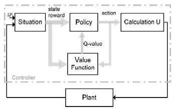
To describe the MFRL scheme (Fig. 1), first the agent is the Policy block and Value Function (VF) block. The VF block updates the table-Q calculated by the Q-learning algorithm. The Policy block selects the best action by the epsilon-greedy algorithm and sends it to the calculation block. The situation block generates the new state by deviation of control variable and set-point. The calculation block computes the control signal generated by the new action. These four blocks form the MFRL scheme. The plant block is the environment and all the blocks form a closed-loop feedback system [4], [10].
B. Q-Learning Algorithm
The Q-learning (QL) algorithm is a simple incremental algorithm developed from the theory of dynamic programming for RL [2]. The QL algorithm developed for the learning agent is as follows:
Step 1: Observe the state $ s_t $, according to the action-state value function, select an action $ a_t $ from the set of available actions in the state set by the epsilon-greedy policy.
Step 2: Calculate control signal $ u_t $ using Eq. (12), and send to the actuator.
$$
u_t = u_{t-1} + \Delta u(a_t) \tag{12}
$$
Observe next state $ s_{t+1} $.
Step 3: Find the maximum action-value function of the next state $ s_{t+1} $, i.e., $ \max_a Q(s_{t+1}, a) $, update the entry in the table for state $ s_t $ and action $ a_t $, and save it at $ Q(s_t, a_t) $ using Eq. (13):
$$
Q(s_t, a_t) = Q(s_t, a_t) + \alpha \left[ r_{t+1} + \gamma \max_a Q(s_{t+1}, a) - Q(s_t, a_t) \right] \tag{13}
$$
Under the state $ s_t $, $ a_t $ is a numerical value of the wait action and the gain $ \alpha $ is a tuning parameter. $ \gamma $ is a discount factor used to weight near reinforcement term heavily than distant one in future actions. When $ \alpha $ is small, the agent learns to behave only for a short-term reward, for instance, if $ \gamma $ is closer to 1, the weight assigned to the long-term reinforcement learning becomes big. $ \alpha $ is a learning rate, and $ 0 < \alpha \leq 1 $ is a tuning parameter that can be used to optimize the speed of learning [4]. $ A_s $ is the set of possible actions in the next available state [4]. $ Q(s_t, a_t) $ is defined as follows. At time step $ t $, the action-value function approximates the expected value of $ r_t $ upon executing $ a_t $ when $ s_t $ is observed, acting optimally thereafter:
$$
Q(s_t, a_t) = \mathbb{E}[r_t | s_t = s, a_t = a] \tag{14}
$$
$$
r_t = \sum_{k=0}^{\infty} \gamma^k r_{t+k+1} \tag{15}
$$
IV. CONTROLLER DESIGN BASED ON REINFORCEMENT LEARNING
A. Control Scheme
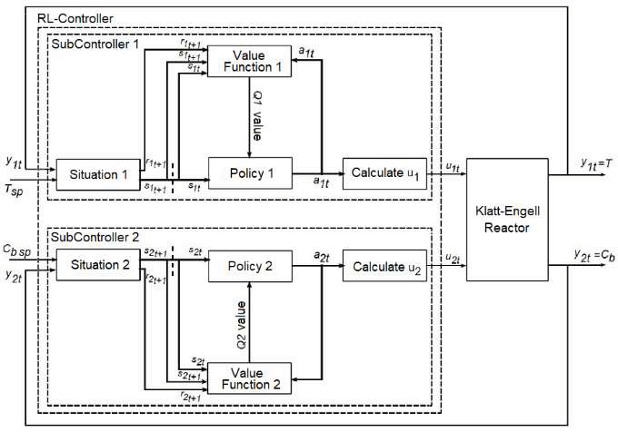
The scheme is based on a double MFRL architecture. TITO systems are interesting because they have interaction with each other. The control system scheme is presented in Figure 2.
B. Q-Learning: States, Actions, and Rewards
The elements of the controller include the following: reactor temperature $ T $, set-point $ T_{sp} $, previous value $ T_{prev} $, product component $ C_B $, set-point $ C_{B,sp} $, previous value $ C_{B,prev} $, QL matrices $ Q_1 $ and $ Q_2 $, states, actions, and control signals. The deviation of states ranges is $ \pm 0.5\ ^\circ C $ for $ s_T $ and $ \pm 0.05\ mol/L $ for $ s_C $. The values of states and actions are given in Tables III and IV respectively.
TABLE III
Definition of States Values
| Index | Temperature State Range ($ ^\circ C $) | Index | Component B State Range (mol/L) |
|---|---|---|---|
| 1 | [87, 88.5) | 1 | [0.75, 0.8) |
| 2 | [88.5, 89) | 2 | [0.8, 0.85) |
| 3 | [89, 89.5) | 3 | [0.85, 0.9) |
| 4 | [89.5, 90) | 4 | [0.9, 0.95) |
| 5 | [90, 90.5) ∪ (90.5, 91] | 5 | [0.95, 1.0) |
| 6 | — | 6 | [1.0, 1.05) |
| 7 | [91, 91.5) | 7 | [1.05, 1.1) |
| 8 | [91.5, 92) | 8 | [1.1, 1.15) |
| 9 | [92, 92.5) ∪ (92.5, 93] | 9 | [1.15, 1.2) |
| 10 | — | 10 | [1.2, 1.2] |
| 11 | [93, 93.5) | 11 | [1.2, 1.25) |
| 12 | [93.5, 94) ∪ (94, 94.5] | 12 | [1.25, 1.3) |
| 13 | [94.5, 95.5) | 13 | [1.3, 1.35) ∪ (1.35, 1.4] |
| 14 | [95.5, 96.5) | 14 | — |
| 15 | [96.5, 97.5) | 15 | [1.4, 1.45) |
| 16 | [97.5, 98.5) | 16 | [1.45, 1.5) |
| 17 | [98.5, 99.5) | 17 | [1.5, 1.55) |
| 18 | [99.5, 100.5) | 18 | — |
| 19 | [100.5, 101.5) | 19 | — |
| 20 | 101.5 | 20 | — |
| 21 | * | 21 | — |
TABLE IV
Definition of Actions Values
| Action Index | $ \Delta u_1 $ (L/s) | Action Index | $ \Delta u_2 $ (kJ/s) | Action Index | $ \Delta u_1 $ (L/s) | Action Index | $ \Delta u_2 $ (kJ/s) |
|---|---|---|---|---|---|---|---|
| 1 | 0.5 | 12 | — | 1 | -0.95 | 13 | -0.45 |
| 2 | 7.5 | 13 | 23.0 | 2 | -0.9 | 14 | -0.4 |
| 3 | 0.9 | 14 | 24.0 | 3 | -0.85 | 15 | -0.35 |
| 4 | 11.0–13.0 | 15–17 | 26.0 | 4 | -0.8 | 16 | -0.3 |
| 5 | 12.5 | 18 | 27.0 | 5 | -0.75 | 17 | -0.25 |
| 6 | 14.0 | 19 | 28.0 | 6 | -0.7 | 18 | -0.2 |
| 7 | — | — | 30.0 | 7 | — | — | -0.15 |
| 8–9 | 15.0–16.0 | 20–21 | 32.0 | 8 | -0.6 | 20 | -0.1 |
| 10 | 17.0 | 22 | 33.0–35.0 | 9 | -0.55 | 21 | 0 |
| 11 | 19.0 | 23 | 36.0 | 10 | -0.5 | — | — |
| — | — | — | — | 11 | -0.45 | — | — |
State deviation is required to compute equation (16):
$$
\delta_T(t) = T_{sp}(t) - T(t) \tag{16}
$$
$$
\delta_C(t) = C_{B,sp}(t) - C_B(t) \tag{17}
$$
Action value scaled to the volume of the reactor and to compute the change of heat flow — are important to compute the control signals via equations (18–19):
$$
u_1(t) = u_{1,prev} + \Delta u_1(a_t) \tag{18}
$$
$$
u_2(t) = u_{2,prev} + \Delta u_2(a_t) \tag{19}
$$
The objective of the control task is to maintain the process around the set-points with a deviation $ \delta_T $ of $ T $ within [-0.125, +0.125] °C (upper) and [-0.125, +0.125] °C (lower), deviation $ \delta_C $ of $ C_B $ within [-0.005, +0.005] mol/L (upper) and [-0.005, +0.005] mol/L (lower), i.e., to maintain the process in state 11 (goal state or set-point state) of $ s_T $ and $ s_C $, and return it to state 11 of $ s_T $ and $ s_C $ despite the occurrence of any disturbance of nonlinear behavior in the plant. To achieve this, a rewards function is introduced when the current states are closer to the set-points compared with the previous states. This rewards function $ R_T $ and $ R_C $ are applied to all states, as shown in equations (20–21):
$$
R_T =
\begin{cases}
-100 & \text{if } |\delta_T| > 0.125 \
-10 \cdot |\delta_T| & \text{otherwise}
\end{cases}
\tag{20}
$$
$$
R_C =
\begin{cases}
-100 & \text{if } |\delta_C| > 0.005 \
-10 \cdot |\delta_C| & \text{otherwise}
\end{cases}
\tag{21}
$$
C. Reference Functions
The simulation is performed for two reference functions. In the first case, they are step inputs shown in equations (22–23). In the second case, the references are sinusoidal functions shown in equations (24–25).
$$
T_{sp}(t) =
\begin{cases}
90.5\ ^\circ C, & t < 2500\ s \
91.5\ ^\circ C, & 2500 \leq t < 5000\ s \
90.5\ ^\circ C, & 5000 \leq t < 7500\ s \
91.5\ ^\circ C, & t \geq 7500\ s
\end{cases}
\tag{22}
$$
$$
C_{B,sp}(t) =
\begin{cases}
1.0\ mol/L, & t < 2500\ s \
1.1\ mol/L, & 2500 \leq t < 5000\ s \
1.0\ mol/L, & 5000 \leq t < 7500\ s \
1.1\ mol/L, & t \geq 7500\ s
\end{cases}
\tag{23}
$$
$$
T_{sp}(t) = 91 + 0.5 \sin\left(\frac{2\pi t}{1000}\right)\ ^\circ C \tag{24}
$$
$$
C_{B,sp}(t) = 1.05 + 0.05 \sin\left(\frac{2\pi t}{1000}\right)\ mol/L \tag{25}
$$
V. SIMULATIONS DETAILS AND DISCUSSIONS OF RESULTS
The control system is divided into two main sub-controllers: one for reactor temperature and one for component B concentration. Each sub-controller has its own action and uses a Q-learning algorithm with a Q-table. The system has 21 states and 21 actions for each sub-controller.
For comparison purposes, the response of two conventional PID controllers is added with the following parameters: the first controller has proportional gain $ K_p = -10 $, integral gain $ K_i = 1 $, and derivative gain $ K_d = -0.001 $; the second controller has $ K_p = -10 $, $ K_i = 1 $, and $ K_d = 0 $. These PID parameters have been obtained using the Auto-tuning PID Simulink tool of MATLAB applied to linear and nonlinear models of the plant. Also, the same parameters have been tested for sinusoidal reference and had an appropriate response in execution.
Applying the above characteristics to reference step variables by equations (22–25), the results are shown in Figures 3–7.
 for Reactor Temperature)
 for Component B)
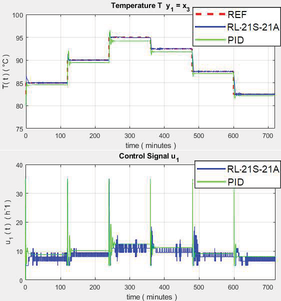
The results in Figure 3 show that the response of $ T $ is enhanced by the RL controller as it responds appropriately according to the reference stepped input, while the conventional PID control exhibits oscillation at the start of the transient response and a large steady-state error. The control signal shows that the RL controller responds naturally to the input change while the PID control signal presents saturation in step changes and is not able to capture the nonlinearity of the process.
 for Reactor Temperature)
 for Component B)
The RL controller responds with overshoots in the phase change, but reaches the value appropriately according to the reference following the input, while the conventional PID control presents overshoot and exhibits a large error in the steady state and is not able to follow the input. The control signal shows that the RL controller responds well, while the PID control signal exhibits overshoots in step changes.
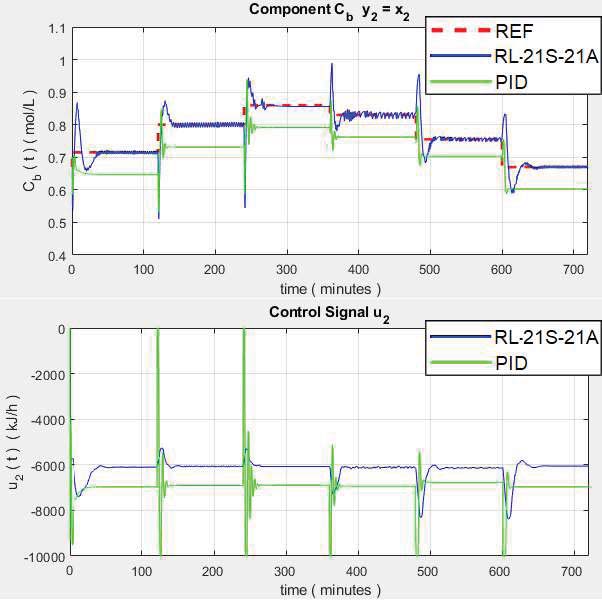
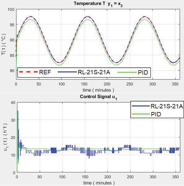
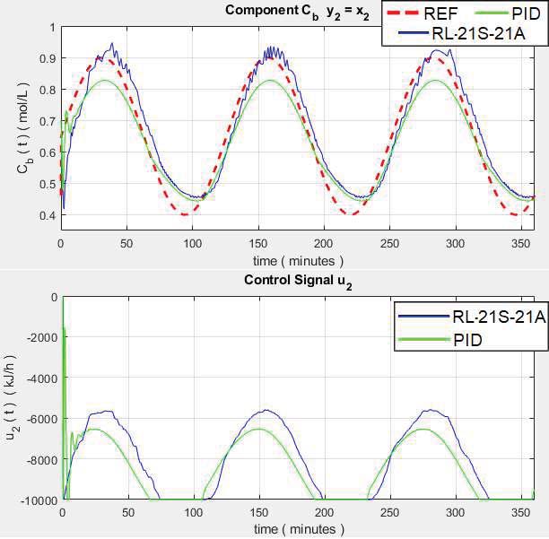
The results in Figure 6 reveal the response of $ C_B $. The RL controller responds correctly according to the sinusoidal reference path, whereas the conventional PID control presents a slightly delayed slight response. The control signal shows that both RL and PID controllers have good performance in the control signal.
for Component B)
The results in Figure 7 reveal for the response of $ C_B $. The RL controller responds with a very small error with respect to the sinusoidal reference trajectory while the conventional PID control does not track the sinusoidal curve producing a delayed response. The control signal shows that the reinforcement learning-based controller responds better than the PID controller.
Table V presents the Root Mean Square Error (RMSE) of the two cases.
TABLE V
Summary of Results RMSE
| RMSE $ y_T $ | Step Input | Sinusoidal Input |
|---|---|---|
| RL Controller | 0.4329 | 0.3872 |
| PID Controller | 0.0384 | 0.0369 |
| RMSE $ y_C $ | ||
| RL Controller | 0.3987 | 0.8970 |
| PID Controller | 0.0313 | 0.0358 |
VI. CONCLUSIONS
Reinforcement Learning does not require an exact model and analysis of the plant and it works directly with the nonlinear state equations of states and variables to control, choosing the states, action rewards, and the best parameters of the controller. Additionally, the RL controller can learn even with a lot of noise data. The RL controller achieves good performance in controlling the references of the reactor temperature and product component B. The main advantage of this control scheme is that it allows designing and controlling systems without a detailed understanding of the dynamics. This is due to the fact that RL explores and exploits any nonlinear and noisy environments.


 983
983

 被折叠的 条评论
为什么被折叠?
被折叠的 条评论
为什么被折叠?
 到【灌水乐园】发言


