线性回归与高级回归模型实践：线性和随机采样的 RidgeLASSO 多项式回归

学习内容

1 Ridge/LASSO 多项式回归的实现

Ridge/LASSO 多项式回归理论

多项式回归是一种强大的工具，用于捕捉数据中的非线性关系。其核心思想是通过在原始特征中引入高次项（如 $x^2$、$x^3$等），扩展特征空间，使模型能够拟合更复杂的模式。然而，当特征数量增加或多项式阶数较高时，模型容易变得过于复杂，导致在训练数据上表现良好但在测试数据上泛化能力差，即过拟合。为了解决这一问题，Ridge回归和LASSO回归被引入到多项式回归中，通过正则化来控制模型的复杂度。

Ridge回归（也称为L2正则化）在损失函数中添加一个L2范数惩罚项。其目标函数可以表示为：

$$\underset{\beta }{\min }\left(\sum _{i=1}^n(y_i-\sum _{j=0}^p{\beta }_j{x}_{ij}{)}^2+\lambda \sum _{j=1}^p{\beta }_j^2\right)$$

其中，$y_i$ 是目标值，$x_{i}j$ 是特征值，${\beta }_j$ 是模型系数，$\lambda$ 是正则化参数，用于控制惩罚强度。L2正则化通过缩小系数的大小来防止过拟合，但不会将系数完全置为零。这使得Ridge回归在处理多重共线性问题时特别有效，因为它通过收缩系数来稳定模型。

LASSO回归（也称为L1正则化）则在损失函数中添加一个L1范数惩罚项。其目标函数为：

$$\underset{\beta }{\min }\left(\sum _{i=1}^n(y_i-\sum _{j=0}^p{\beta }_j{x}_{ij}{)}^2+\lambda \sum _{j=1}^p|{\beta }_j|\right)$$

L1正则化的独特之处在于它能够将一些系数压缩为零，从而实现特征选择。这对于高维数据集尤其有用，因为它可以帮助我们识别最重要的特征，并简化模型。

在多项式回归中结合Ridge或LASSO正则化，可以有效地平衡模型的偏差和方差。通过调整正则化参数 $\lambda$，我们可以控制模型的复杂度，找到一个在训练数据和测试数据上表现都较好的模型。这种结合方式在处理具有复杂非线性关系的数据时特别有效，为数据分析提供了强大的工具。

1.1 导入库

导入NumPy（数值计算）、Pandas（数据处理）和Matplotlib（绘图）三个Python科学计算核心库

%pip install scikit-learn==1.1.3

import numpy as np
import pandas as pd
import matplotlib.pyplot as plt
from sklearn.preprocessing import PolynomialFeatures
from sklearn.pipeline import make_pipeline
from sklearn.linear_model import LassoCV
from sklearn.metrics import mean_squared_error
from sklearn.linear_model import LinearRegression
from sklearn.linear_model import LassoCV
from sklearn.linear_model import RidgeCV
from sklearn.ensemble import AdaBoostRegressor
from sklearn.model_selection import train_test_split
from sklearn.pipeline import make_pipeline
%matplotlib inline

1.2 定义程序的全局变量

定义了多项式回归实验的参数：生成41个x值（范围1-10），添加均值为0、标准差为2的高斯噪声；设置岭回归的正则化强度（10到100的等比数列）、Lasso回归的参数（精度0.001，alpha数20，迭代1000次），以及多项式阶数范围（2-8阶）。

N_points = 41 # 构建函数所需的点
x_min = 1 # x（特征）范围的最小值
x_max = 10 # x（特征）范围的最大值
noise_mean = 0 # 高斯噪声添加器的均值
noise_sd = 2 # 高斯噪声添加器的标准差
ridge_alpha = tuple([10**(x) for x in range(-3,0,1) ]) # 岭回归中的正则化强度
lasso_eps = 0.001
lasso_nalpha=20
lasso_iter=1000
degree_min = 2
degree_max = 8

1.3 遵循非线性函数生成特征和输出向量 ¶

$$Thegroundtruthororiginatingfunctionisasfollows:$$

$$y=f(x)=x^2.sin(x).e^{-0.1x}+\psi (x)$$

$$\psi (x)=f(x|\mu ,{\sigma }^2)=\frac{1}{\sqrt{2\pi {\sigma }^2}}{e}^{-\frac{(x-\mu {)}^2}{2{\sigma }^2}}$$

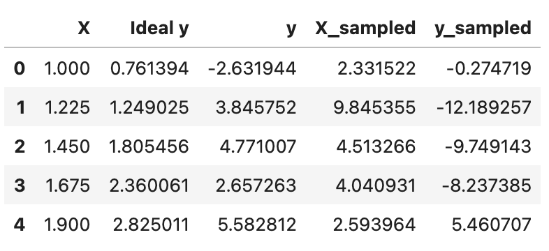
首先生成1001个均匀分布的x值用于平滑曲线绘制，然后创建两组不同的x采样点：41个均匀间隔点和41个均匀随机分布点。定义了一个非线性目标函数$f(x)=x^2\cdot sin(x)\cdot e^{\frac{-1x}{10}}$，并添加高斯噪声生成对应的y值。最后将数据整理为DataFrame，包含均匀x值、理想y值（无噪声）、带噪声的均匀采样y值、随机采样x值及其对应的带噪声y值，并展示前5行数据。

x_smooth = np.array(np.linspace(x_min,x_max,1001))

# 线性间隔采样点
X=np.array(np.linspace(x_min,x_max,N_points))

# 从均匀随机分布中提取的样本
X_sample = x_min+np.random.rand(N_points)*(x_max-x_min)

def func(x):
    result = x**2*np.sin(x)*np.exp(-(1/x_max)*x)
    return (result)

noise_x = np.random.normal(loc=noise_mean,scale=noise_sd,size=N_points)

y = func(X)+noise_x
y_sampled = func(X_sample)+noise_x

df = pd.DataFrame(data=X,columns=['X'])
df['Ideal y']=df['X'].apply(func)
df['y']=y
df['X_sampled']=X_sample
df['y_sampled']=y_sampled
df.head()

1.4 绘制函数，包括理想特征和观察到的输出 （带有过程和观察噪声） ¶

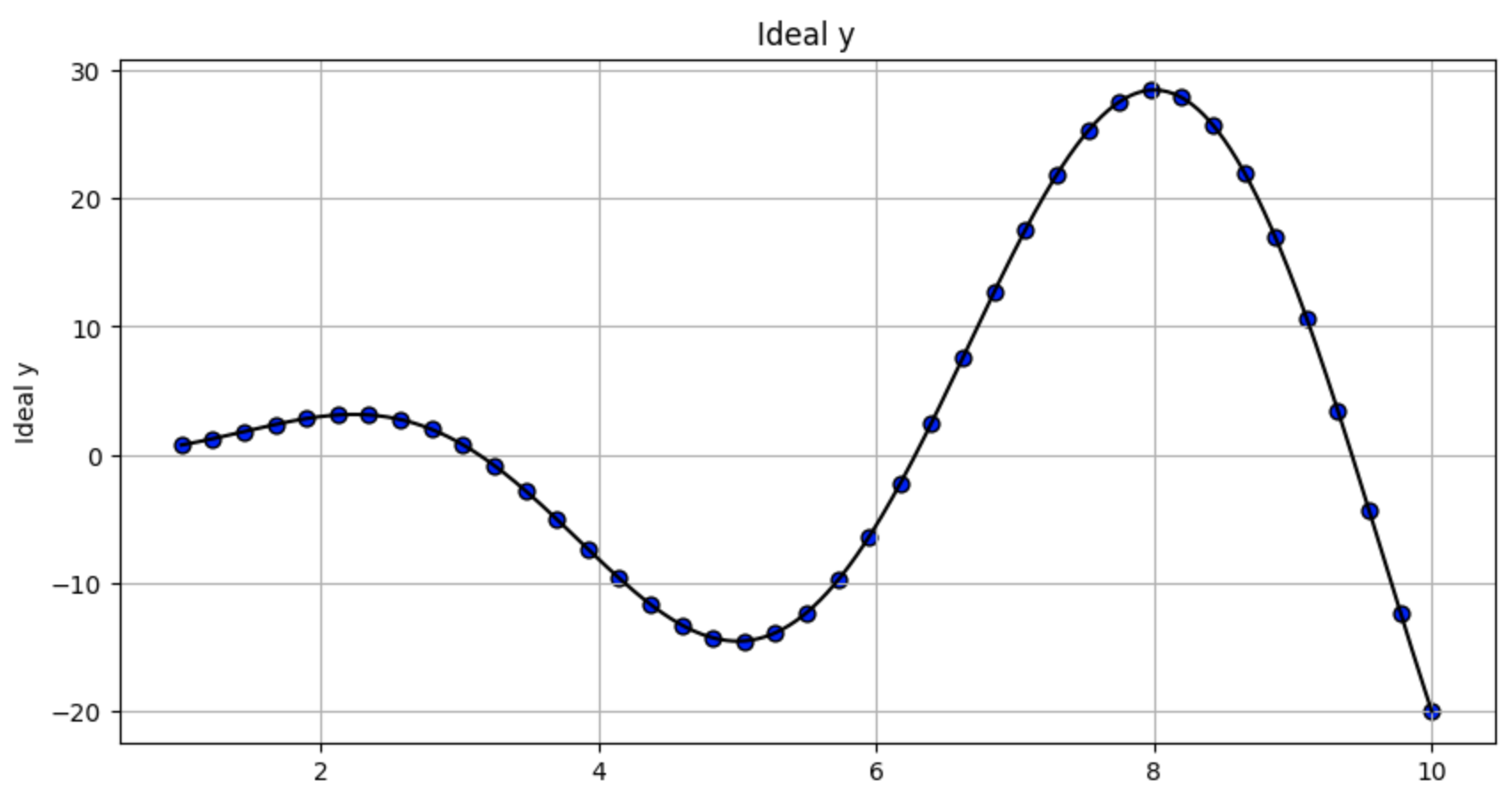
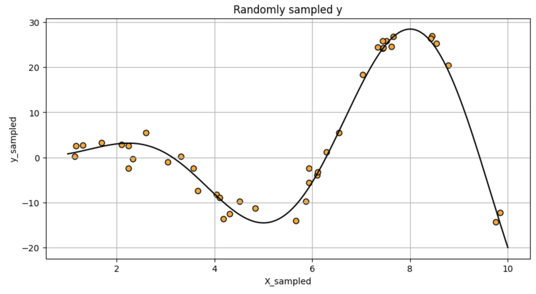
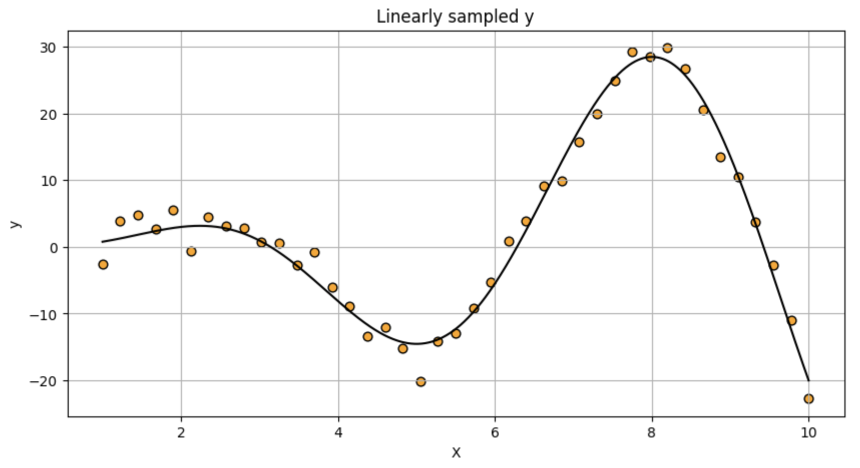
通过三个散点图可视化不同采样方式下的数据分布：

第一个图展示均匀采样点（X）与理想无噪声y值的关系，黑色曲线表示真实函数f(x)=x²·sin(x)·e^(-x/10)。

第二个图显示随机采样点（X_sampled）与带噪声y值的分布，同样叠加真实函数曲线。

第三个图呈现均匀采样点与带噪声y值的关系，也包含真实函数曲线作为参考。

所有图表使用相同可视化参数：网格线、黑色边框、橙色/蓝色散点（随机采样用橙色，均匀采样用蓝色），点大小为40，图像尺寸10x5英寸。这种对比有助于观察采样方式对数据分布和噪声影响的表现。

df.plot.scatter('X','Ideal y',title='Ideal y',grid=True,edgecolors=(0,0,0),c='blue',s=40,figsize=(10,5))
plt.plot(x_smooth,func(x_smooth),'k')

df.plot.scatter('X_sampled',y='y_sampled',title='Randomly sampled y',
                grid=True,edgecolors=(0,0,0),c='orange',s=40,figsize=(10,5))
plt.plot(x_smooth,func(x_smooth),'k')

df.plot.scatter('X',y='y',title='Linearly sampled y',grid=True,edgecolors=(0,0,0),c='orange',s=40,figsize=(10,5))
plt.plot(x_smooth,func(x_smooth),'k')

1.5 导入 scikit-learn 库并准备训练/测试拆分 ¶

导入scikit-learn库中的回归建模工具，将数据集划分为67%训练集和33%测试集，并将一维特征数组重塑为二维格式以满足scikit-learn的输入要求。

X_train, X_test, y_train, y_test = train_test_split(df['X'], df['y'], test_size=0.33)
X_train=X_train.values.reshape(-1,1)
X_test=X_test.values.reshape(-1,1)

1.6 多项式模型使用岭正则化通过（pipelined）完成样本的等距分布

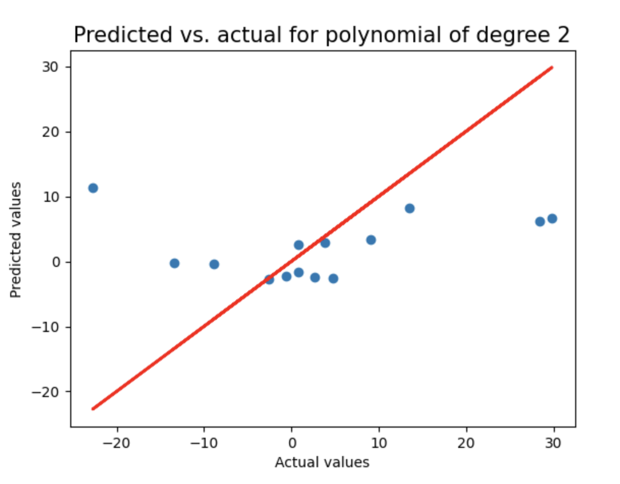
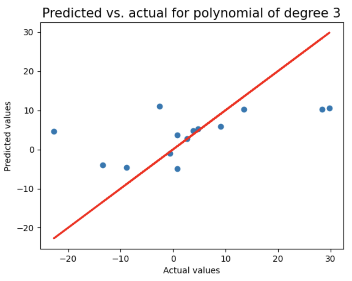
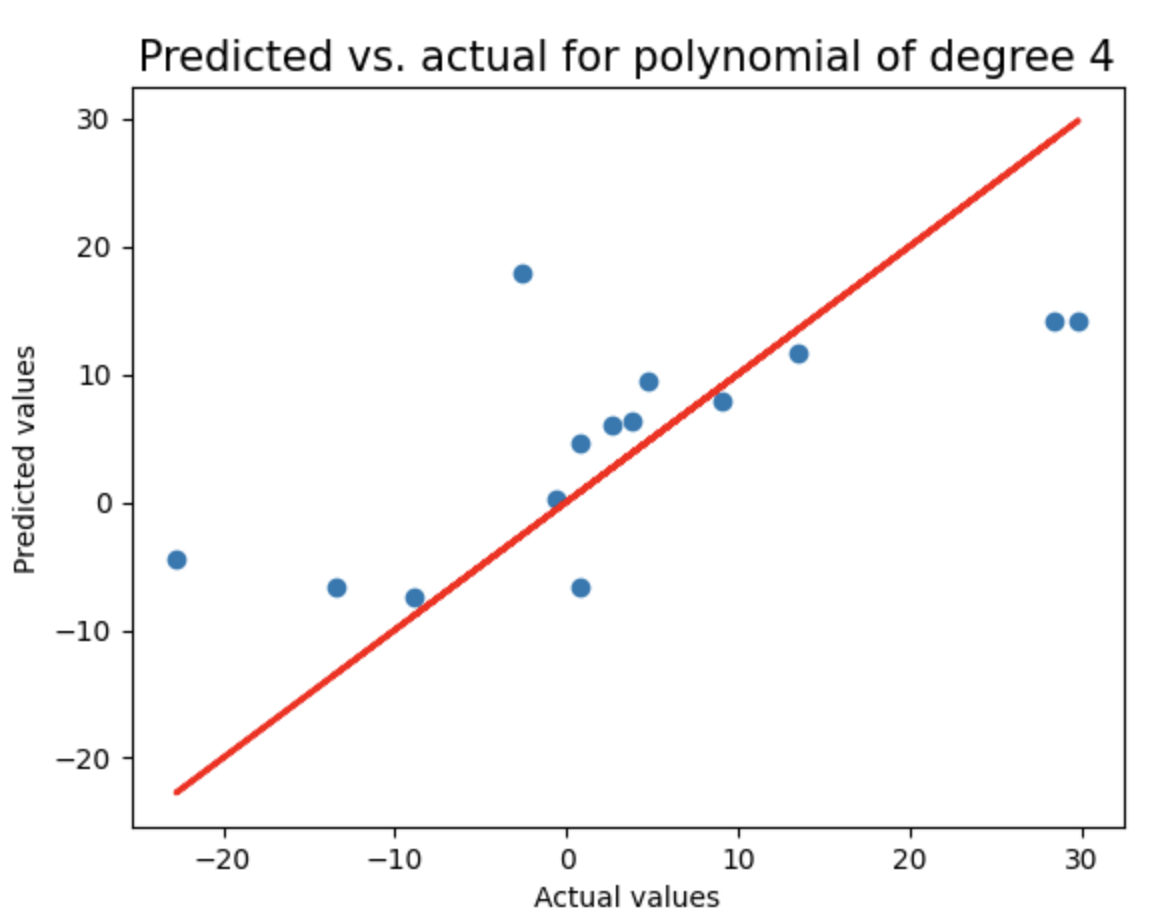
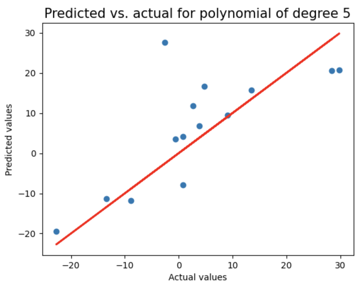
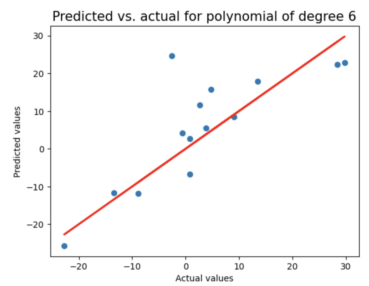
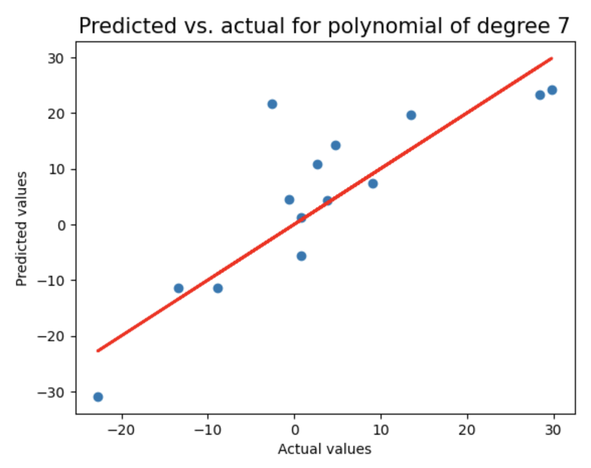
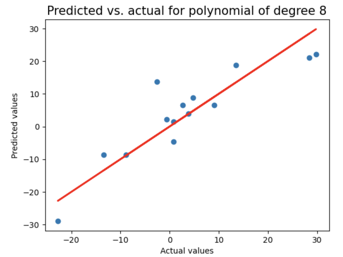
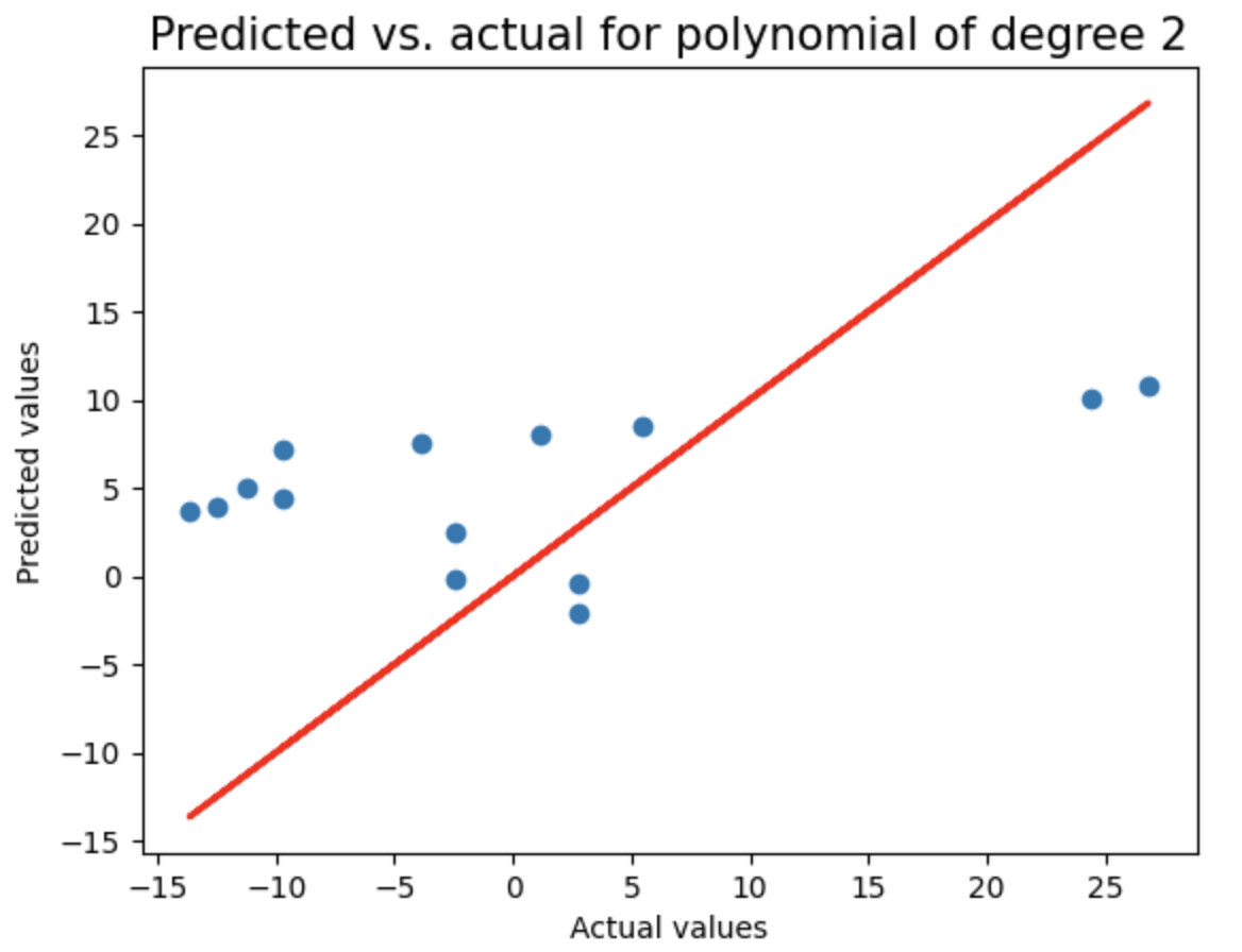
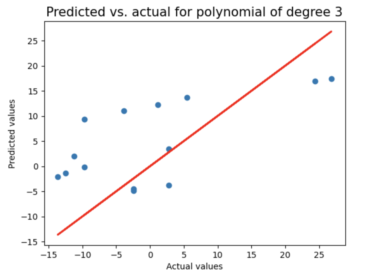
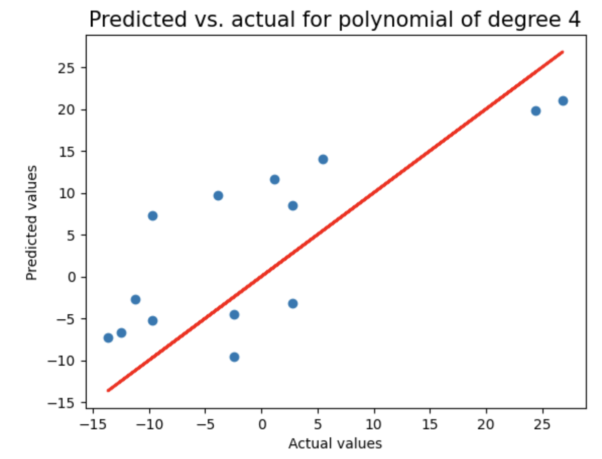
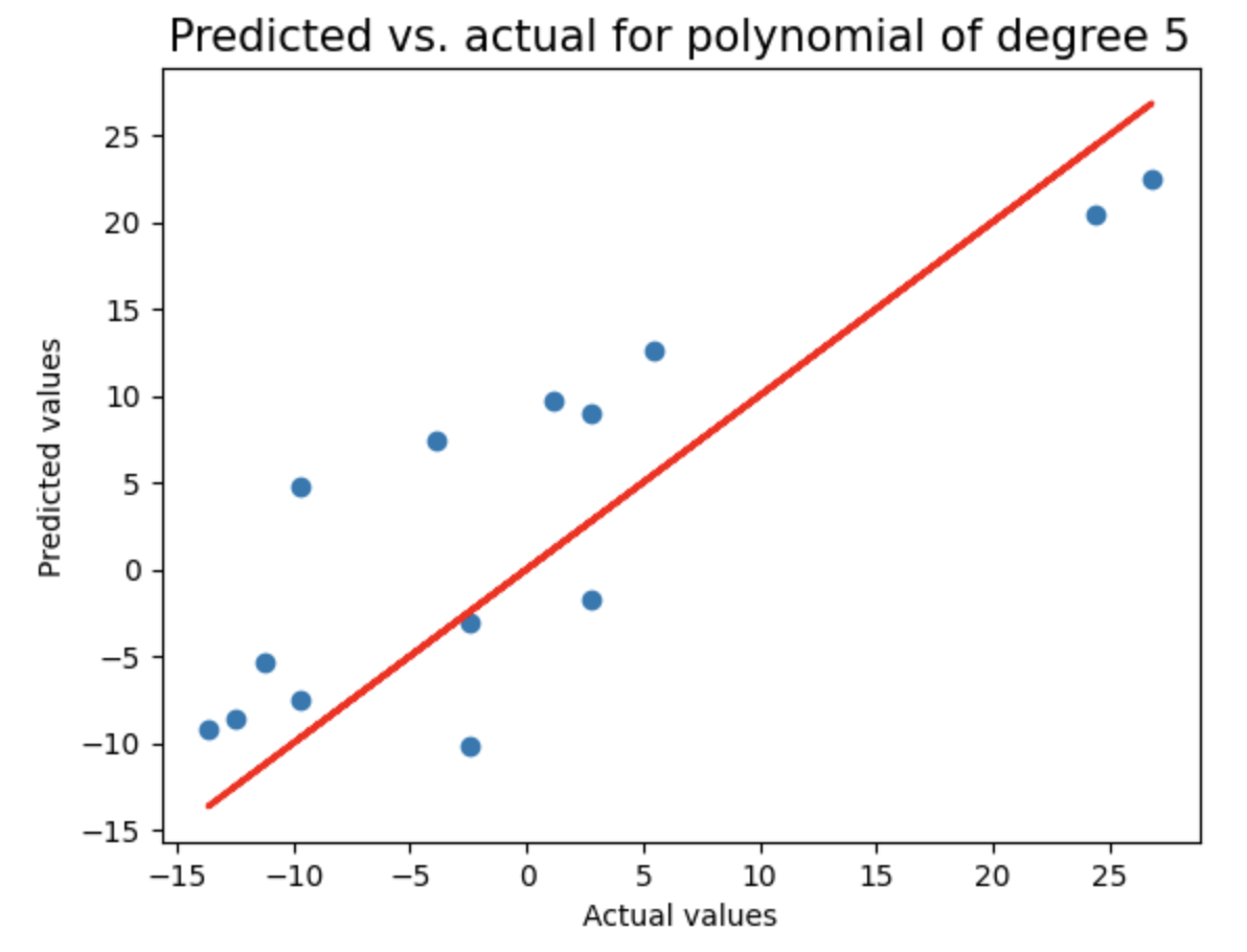
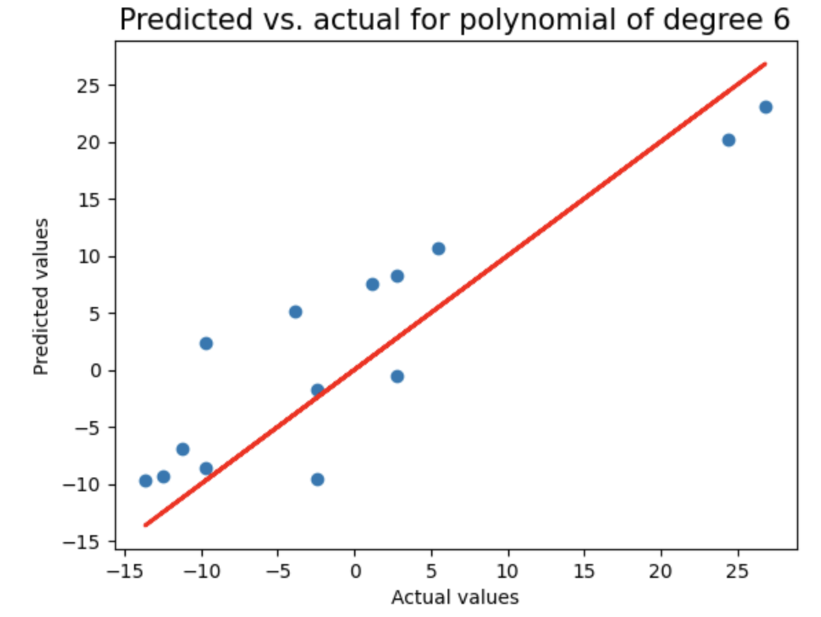
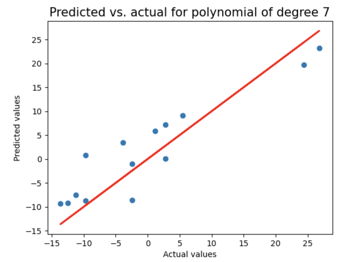
这是一种先进的机器学习方法，通过惩罚高值系数（即保持它们有界）来防止过度拟合。通过循环测试2到8阶多项式回归模型，使用LassoCV进行正则化，记录每个模型的测试集R²分数和多项式阶数，并绘制预测值与实际值的对比图（含理想预测线），用于评估不同复杂度模型的泛化性能。

linear_sample_score = []
poly_degree = []
for degree in range(degree_min,degree_max+1):
    
    model = make_pipeline(PolynomialFeatures(degree), LassoCV(eps=lasso_eps,n_alphas=lasso_nalpha, 
                                                                  max_iter=lasso_iter,normalize=True,cv=5))
   
    model.fit(X_train, y_train)
    y_pred = np.array(model.predict(X_train))
    test_pred = np.array(model.predict(X_test))
    RMSE=np.sqrt(np.sum(np.square(y_pred-y_train)))
    test_score = model.score(X_test,y_test)
    linear_sample_score.append(test_score)
    poly_degree.append(degree)
    print("Test score of model with degree {}: {}\n".format(degree,test_score))

    plt.figure()
    plt.title("Predicted vs. actual for polynomial of degree {}".format(degree),fontsize=15)
    plt.xlabel("Actual values")
    plt.ylabel("Predicted values")
    plt.scatter(y_test,test_pred)
    plt.plot(y_test,y_test,'r',lw=2)

linear_sample_score

Result:

[0.01972262259273616,
 0.31696961499861065,
 0.48354017207617983,
 0.4619441805300364,
 0.5614210750057387,
 0.6263648368163351,
 0.7935722818093062]

1.7 使用随机采样对数据集建模 ¶

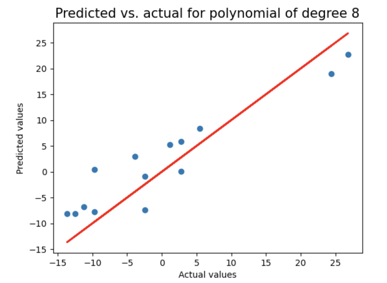
对随机采样数据执行与之前相同的分析：将数据划分为训练集和测试集，测试2到8阶多项式回归模型，使用LassoCV进行正则化，记录每个模型的测试集R²分数和多项式阶数，并绘制预测值与实际值的对比图，用于评估不同复杂度模型在随机采样数据上的泛化性能。

X_train, X_test, y_train, y_test = train_test_split(df['X_sampled'], df['y_sampled'], test_size=0.33)
X_train=X_train.values.reshape(-1,1)
X_test=X_test.values.reshape(-1,1)


random_sample_score = []
poly_degree = []
for degree in range(degree_min,degree_max+1):
   
    model = make_pipeline(PolynomialFeatures(degree), LassoCV(eps=lasso_eps,n_alphas=lasso_nalpha, 
                                                                  max_iter=lasso_iter,normalize=True,cv=5))
  
    model.fit(X_train, y_train)
    y_pred = np.array(model.predict(X_train))
    test_pred = np.array(model.predict(X_test))
    RMSE=np.sqrt(np.sum(np.square(y_pred-y_train)))
    test_score = model.score(X_test,y_test)
    random_sample_score.append(test_score)
    poly_degree.append(degree)
    
    print("Test score of model with degree {}: {}\n".format(degree,test_score))

    
    plt.figure()
    plt.title("Predicted vs. actual for polynomial of degree {}".format(degree),fontsize=15)
    plt.xlabel("Actual values")
    plt.ylabel("Predicted values")
    plt.scatter(y_test,test_pred)
    plt.plot(y_test,y_test,'r',lw=2)

random_sample_score

Result:

[0.0037787102872796074,
 0.26633554841881124,
 0.5084485116234183,
 0.6629824255648642,
 0.7732499623544961,
 0.8294830115060845,
 0.8342525581964225]

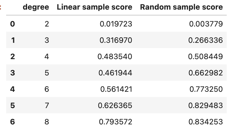
df_score = pd.DataFrame(data={'degree':[d for d in range(degree_min,degree_max+1)],
                              'Linear sample score':linear_sample_score,
                              'Random sample score':random_sample_score})
df_score

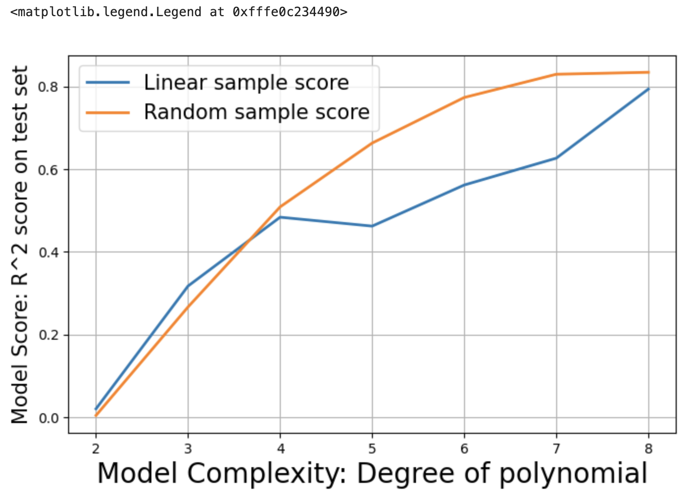
plt.figure(figsize=(8,5))
plt.grid(True)
plt.plot(df_score['degree'],df_score['Linear sample score'],lw=2)
plt.plot(df_score['degree'],df_score['Random sample score'],lw=2)
plt.xlabel("Model Complexity: Degree of polynomial",fontsize=20)
plt.ylabel("Model Score: R^2 score on test set",fontsize=15)
plt.legend(['Linear sample score','Random sample score'],fontsize=15)

1.8 从交叉验证的模型管道中引入正则化强度 ¶

从已训练的scikit-learn管道模型中提取Lasso回归器（model.steps[1][1]），并访问其alpha_属性，该属性表示通过交叉验证选择的最佳正则化强度参数。

m=model.steps[1][1]
m.alpha_

Output:
0.004868836133537874