Camera Calibration [相机标定-张正友]

From：Blog

1. camera model

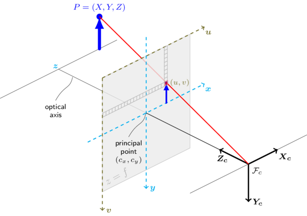
• $X_c{Y}_c{Z}_c$ : camera coordinate system
• $uv$: pixel coordinate system, [dimension in pixel]
• $xy$: image coordinate system, [dimension in mm]
• $XYZ$: word coordinate system, [dimension in pixel]

2. $XYZ\Rightarrow X_c{Y}_c{Z}_c$

the main process is to transform points in word coordinate system $XYZ$ into camera coordinate system $X_c{Y}_c{Z}_c$, this process is done with a rotation and shift matrix
$$\left[\begin{array}{c}{x}_c\\ y_c\\ z_c\\ 1\end{array}\right]=\left[\begin{array}{cc}R& T\\ 0& 1\end{array}\right]\left[\begin{array}{c}{x}_w\\ y_w\\ x_w\\ 1\end{array}\right]$$
where $R$ is the rotation matrix
$$R=\left[\begin{array}{ccc}{r}_{11}& r_{12}& r_{13}\\ r_{21}& r_{22}& r_{23}\\ r_{31}& r_{32}& r_{33}\end{array}\right]$$
and $T$ is the shift vector
$$T={\left[\begin{array}{ccc}{t}_x& t_y& t_z\end{array}\right]}^T$$

3. $X_c{Y}_c{Z}_c\Rightarrow xy$

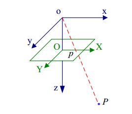
After transformed in camera coordinate system, we can project the points into the image plane using pinhole model. suppose the point $p_c=(x_c,y_c,z_c{)}^T$ in camera coordinate system, then it’s coordinate in image plane can be obtained as the follow:
$$\frac{x}{x_w}=\frac{y}{y_w}=\frac{f}{z_w}$$
so
$$\{\begin{array}{rl}x& =\frac{f{x}_c}{z_c}\\ y& =\frac{f{y}_c}{z_c}\end{array}$$

thus
$$z_c\left[\begin{array}{c}x\\ y\\ 1\end{array}\right]=\left[\begin{array}{cccc}f& 0& 0& 0\\ 0& f& 0& 0\\ 0& 0& 1& 0\end{array}\right]\left[\begin{array}{c}{x}_c\\ y_c\\ z_c\\ 1\end{array}\right]$$

4. $xy\Rightarrow uv$

4.1 condition: $u\perp v$

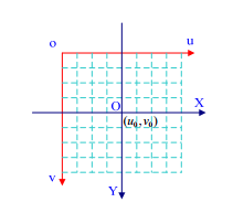
usually, the origin point of pixel coordinate system is located in the top left corner while the origin of image coordinate system is located in the center of the image plane, causing a shift vector $(u_0,v_0)$ between this two coordinate system.

Denoted the size of each pixel in $u,v$ direction as $dx,dy$ (dimension in mm). then we can get the relationship between them.
$$\left[\begin{array}{c}u\\ v\\ 1\end{array}\right]=\left[\begin{array}{ccc}\frac{1}{dx}& 0& u_0\\ 0& \frac{1}{dy}& v_0\\ 0& 0& 1\end{array}\right]\left[\begin{array}{c}x\\ y\\ 1\end{array}\right]$$

4.2 condition: $u/\perp v$

In this condition, the matrix is a little complex but still easy to understand
$$\{\begin{array}{rl}u& =\frac{x-ycot\theta }{dx}+u_0\\ v& =\frac{y}{dysin\theta }+v_0\end{array}$$
thus
$$\begin{array}{rl}\left[\begin{array}{c}u\\ v\\ 1\end{array}\right]& =\left[\begin{array}{ccc}\frac{1}{dx}& -\frac{1}{d_{x}tan\theta }& u_0\\ 0& \frac{1}{dysin\theta }& v_0\\ 0& 0& 1\end{array}\right]\left[\begin{array}{c}x\\ y\\ 1\end{array}\right]\\ & =\left[\begin{array}{ccc}{\alpha }_x& c& u_0\\ 0& {\alpha }_y& v_0\\ 0& 0& 1\end{array}\right]\left[\begin{array}{c}x\\ y\\ 1\end{array}\right]\end{array}$$

5. relation

Through the analysis of above, the relationship between world and pixel coordinate system can be written as follows:
$$\begin{array}{rl}{z}_c\left[\begin{array}{c}u\\ v\\ 1\end{array}\right]& =\left[\begin{array}{cccc}{\alpha }_x& c& u_0& 0\\ 0& {\alpha }_y& v_0& 0\\ 0& 0& 1& \end{array}\right]\left[\begin{array}{cccc}f& 0& 0& 0\\ 0& f& 0& 0\\ 0& 0& 1& 0\end{array}\right]\left[\begin{array}{cc}R& T\\ 0& 1\end{array}\right]\left[\begin{array}{c}{x}_w\\ y_w\\ x_w\\ 1\end{array}\right]\\ & =\left[\begin{array}{cccc}{\alpha }_x& c& u_0& 0\\ 0& {\alpha }_y& v_0& 0\\ 0& 0& 1& 0\end{array}\right]\left[\begin{array}{cc}R& T\\ 0& 1\end{array}\right]\left[\begin{array}{c}{x}_w\\ y_w\\ x_w\\ 1\end{array}\right]\\ & =M_1{M}_2{X}_w\\ & =M{X}_w\end{array}$$
where ${\alpha }_x=f/dx$ and ${\alpha }_y=f/dy$ is called scale factors in image $u$ and $v$ axes, $M_1$ is called camera intrinsic matrix, $M_2$ is called camera extrinsic parameters,c is the parameter describing the skewness of the two image axes.

6. Camera Calibration

6.1. general conception

The method is proposed by Zhengyou Zhang which only require a camera to observe a planar patttern at a few (at least two) different orientations.

In order to keep equations consistent with the paper written by Zhengyou Zhang, here the transformation matrix is rewritten as the follow.
$$s\tilde{m}=A\left[\begin{array}{cc}R& t\end{array}\right]\tilde{M}$$
where $\tilde{m}={\left[\begin{array}{c}u,v,1\end{array}\right]}^T$ represent the 2D point and $\tilde{M}={\left[\begin{array}{c}X,Y,Z,1\end{array}\right]}^T$ represent the corresponding 3D point and
$$A=\left[\begin{array}{ccc}\alpha & c& u_0\\ 0& \beta & v_0\\ 0& 0& 1\end{array}\right]$$
To calibrate the camera, the model plane was assumed to be $Z=0$, then
$$s\left[\begin{array}{c}u\\ v\\ 1\end{array}\right]=A\left[\begin{array}{cccc}{r}_1& r_2& r_3& t\end{array}\right]\left[\begin{array}{c}X\\ Y\\ 0\\ 1\end{array}\right]=A\left[\begin{array}{ccc}{r}_1& r_2& t\end{array}\right]\left[\begin{array}{c}X\\ Y\\ 1\end{array}\right]$$
according to the above equation, $\tilde{M}={\left[\begin{array}{c}X,Y,1\end{array}\right]}^T$ is defined in the following part. therefore, the homography matrix $H$ is induced.
$$s\tilde{m}=H\tilde{M}$$
where
$$H=A\left[\begin{array}{ccc}{r}_1& r_2& t\end{array}\right]$$

6.2. Estimation of the homography matrix $H$

$M_i$ and $m_i$ respectively represent the model and image points. According to maximum likelihood method, the object function should be minimized.
$$\sum _i(m_i-\widehat{m_i}{)}^T{\Lambda }^{-1}(m_i-\widehat{m_i})$$
where
$$\widehat{m_i}=\frac{1}{\overline{h_3}{M}_i}\left[\begin{array}{c}\overline{h_1}{M}_i\\ \overline{h_2}{M}_i\end{array}\right]$$
$\overline{h_i}$ is the $i^{th}$ row of H, assuming ${\Lambda }_{m_i}={\sigma }^{2}I$ for all $i$, thus, $\sum _i||m_i-\widehat{m_i}|{|}^2$ should be minimized. The Levenberg-Marquardt algorithm was implemented and initial guess can be obtained as follows:

Let $x=[\overline{h_1^T},\overline{h_2^T},\overline{h_3^T}{]}^T$. then $s\tilde{m}=H\tilde{M}$ can be rewritten as
$$\left[\begin{array}{ccc}{\tilde{M}}^T& 0^T& -u{\tilde{M}}^T\\ 0^T& {\tilde{M}}^T& -v{\tilde{M}}^T\end{array}\right]x=0$$
for example
$$s\left[\begin{array}{c}{u}_i\\ v_i\\ 1\end{array}\right]=\left[\begin{array}{ccc}{h}_{11}& h_{12}& h_{13}\\ h_{21}& h_{22}& h_{23}\\ h_{31}& h_{32}& h_{33}\end{array}\right]\left[\begin{array}{c}{x}_{wi}\\ y_{wi}\\ 1\end{array}\right]$$
that is
$$\{\begin{array}{ll}{h}_{11}{x}_{wi}+h_{12}{y}_{wi}+h_{13}-h_{31}{x}_{wi}{u}_i-h_{32}{y}_{wi}{u}_i-h_{33}{u}_i& =0\\ h_{21}{x}_{wi}+h_{22}{y}_{wi}+h_{23}-h_{31}{x}_{wi}{v}_i-h_{32}{y}_{wi}{v}_i-h_{33}{v}_i& =0\end{array}$$
assuming $h_{33}=1$, because there is no impact on the matrix $H$, this assumes just scale the matrix $H$. so we have
$$\left[\begin{array}{ccccccccc}{x}_{wi}& y_{wi}& 1& 0& 0& 0& -u_i{x}_{wi}& -u_i{y}_{wi}& -u_i\\ 0& 0& 0& x_{wi}& y_{wi}& 1& -v_i{x}_{wi}& -v_i{y}_{wi}& -v_i\end{array}\right]\left[\begin{array}{c}{h}_{11}\\ h_{12}\\ h_{13}\\ h_{21}\\ h_{22}\\ h_{23}\\ h_{31}\\ h_{32}\\ 1\end{array}\right]=0$$
simply, we have $Lx=0$, where $L$ is a $2n\times 9$ matrix. for this equation, SVD method can be used or the eigenvector of $L^{T}L$ can be estimated for this equation. Note that there is one homography matrix for each image and they are different from each other. Since there are 8 unknown parameters, in each image, 4 corresponding points are needed to estimate matrix $H$.

6.3. constraints of intrinsic parameters

denote H as $H=\left[\begin{array}{ccc}h1& h_2& h_3\end{array}\right]$, then
$$\left[\begin{array}{ccc}h1& h_2& h_3\end{array}\right]=\lambda A\left[\begin{array}{ccc}r1& r_2& r_3\end{array}\right]$$
because $r_1$ and $r_2$ are orthonormal, we have
$$\begin{array}{rl}{h}_1^T{A}^{-T}{A}^{-1}{h}_2& =0\\ h_1^T{A}^{-T}{A}^{-1}{h}_1& =h_2^T{A}^{-T}{A}^{-1}{h}_2\end{array}$$
note that there are 8 parameters (3 for rotation, 3 for translation and 2 for intrinsic parameters)

Let
$$\begin{array}{rl}B& =A^{-T}{A}^{-1}=\left[\begin{array}{ccc}{B}_{11}& B_{12}& B_{13}\\ B_{21}& B_{22}& B_{23}\\ B_{31}& B_{32}& B_{33}\end{array}\right]\\ & =\left[\begin{array}{ccc}\frac{1}{{\alpha }_x^2}& -\frac{c}{{\alpha }_x^2{\alpha }_y}& \frac{c{v}_0-u_0{\alpha }_y}{{\alpha }_x^2{\alpha }_y}\\ -\frac{c}{{\alpha }_x^2{\alpha }_y}& \frac{c^2}{{\alpha }_x^2{\alpha }_y^2}+\frac{1}{{\alpha }_y^2}& -\frac{c(c{v}_0-u_0{\alpha }_y)}{{\alpha }_x^2{\alpha }_y^2}-\frac{v_0}{{\alpha }_y^2}\\ \frac{c{v}_0-u_0{\alpha }_y}{{\alpha }_x^2{\alpha }_y}& -\frac{c(c{v}_0-u_0{\alpha }_y)}{{\alpha }_x^2{\alpha }_y^2}-\frac{v_0}{{\alpha }_y^2}& \frac{(c{v}_0-u_0{\alpha }_y{)}^2}{{\alpha }_x^2{\alpha }_y^2}+\frac{v_0^2}{{\alpha }_y^2}+1\end{array}\right]\end{array}$$
now, define
$$b=\left[\begin{array}{cccccc}{B}_{11}& B_{12}& B_{22}& B_{13}& B_{23}& B_{33}\end{array}\right]$$
and let the $i^{th}$ column vector of $H$ be $h_i={\left[\begin{array}{c}{h}_{i1},h_{i2},h_{i3}\end{array}\right]}^T$, then
$$h_i^{T}B{h}_j=v_{ij}^{T}b$$
where
$$v_{ij}=\left[\begin{array}{c}{h}_{i1}{h}_{j1},h_{i1}{h}_{j2}+h_{i2}{h}_{j1},h_{i2}{h}_{j2},h_{i3}{h}_{j1}+h_{i1}{h}_{j3},h_{i3}{h}_{j2}+h_{i2}{h}_{j3},h_{i3}{h}_{j3}\end{array}\right]$$
therefore
$$\left[\begin{array}{c}{v}_{12}^T\\ (v_{11}-v_{22}{)}^T\end{array}\right]b=0$$
if n images of the model plane are observed, we have
$$Vb=0$$
where $V$ is a $2n\times 6$ matrix.

if $n\ge 3$, unique value of b will be obtained, if $n=3$, additional constraint $c=0$ can be added to solve the equations. once $b$ is estimated, we can compute the camera intrinsic matrix $A$ as follows
$$\begin{array}{rl}{v}_0& =(B_{12}{B}_{13}-B_{11}{B}_{23})/(B_{11}{B}_{22}-B_{12}^2)\\ \lambda & =B_{33}-[B_{13}^2+v_0(B_{12}{B}_{13}-B_{11}{B}_{23})]/B_{11}\\ \alpha & =\sqrt{\lambda /B_{11}}\\ \beta & =\sqrt{\lambda B_{11}/(B_{11}{B}_{22}-B_{12}^2)}\\ c& =-B_{12}{\alpha }^2\beta /\lambda \\ u_0& =c{v}_0/\alpha -B_{13}{\alpha }^2/\lambda \end{array}$$

6.4 Distortion model

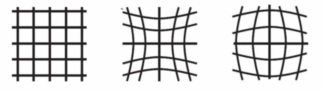
Only the first two terms of radial distortion are considered. Let $(u,v)$ be the ideal (no distorted) pixel image coordinates, and $(\breve{u},\breve{v})$ the corresponding real observed image coordinates. similarly, $(x,y)$ and $(\breve{x},\breve{y})$ are the same meaning. So
$$\begin{array}{rl}\breve{x}& =x+x[k_1(x^2+y^2)+k_2(x^2+y^2{)}^2]\\ \breve{y}& =y+y[k_1(x^2+y^2)+k_2(x^2+y^2{)}^2]\end{array}$$
where $k_1$ and $k_2$ are the coefficients of the radial distortion. thus we have
$$\begin{array}{rl}\breve{u}& =u+(u-u_0)[k_1(x^2+y^2)+k_2(x^2+y^2{)}^2]\\ \breve{v}& =v+(v-v_0)[k_1(x^2+y^2)+k_2(x^2+y^2{)}^2]\end{array}$$
because the distortion is small, we would like to estimate the other parameters followed by estimating $k_1$ and $k_2$
$$\left[\begin{array}{cc}(u-u_0)(x^2+y^2)& (u-u_0)(x^2+y^2{)}^2\\ (v-v_0)(x^2+y^2)& (v-v_0)(x^2+y^2{)}^2\end{array}\right]\left[\begin{array}{c}{k}_1\\ k_2\end{array}\right]=\left[\begin{array}{c}\breve{u}-u\\ \breve{v}-v\end{array}\right]$$
Given $m$ points in $n$ images, we have $2mn$ equations and the matrix $Dk=d$, where $k=[k_1,k_2{]}^T$, and the solution is given by
$$k=(D^{T}D{)}^{-1}{D}^{T}d$$

6.5 Complete Maximum Likelihood Estimation

$$\sum _{i=1}^n\sum _{j=1}^m||m_{i,j}-\breve{m}(A,k_1,k_2,R_i,t_i,M_j)|{|}^2$$

the initial guess of $A$ and { R i , t i ∣ i = 1 , . . n } \{R_i,t_i|i=1,..n\} {Ri​,ti​∣i=1,..n} can be estimated in Sec 6.2 and Sec 6.3. An initial guess of { k i ∣ i = 1 , 2 } \{k_i|i=1,2\} {ki​∣i=1,2} can be obtained in Sec 6.4 or simply set them to zero. the Levevberg-Marquartdt Algorithm is implemented here to solve the nonlinear problem.

---

Reference

[1] Zhang Z . Flexible camera calibration by viewing a plane from unknown orientation[C]// Computer Vision, 1999. The Proceedings of the Seventh IEEE International Conference on. IEEE Computer Society, 1999.

[2] blog: https://www.cnblogs.com/zyly/p/9366080.html

[3] blog: https://blog.youkuaiyun.com/lql0716/article/details/71973318?locationNum=8&fps=1