[ESWA 2023]Multi-scale receptive fields: Graph attention neural network for hyperspectral image cla--优快云博客

①Labelled set of a graph is defined as $\{(\boldsymbol{x}_i,\boldsymbol{y}_i)\}_{i=1}^l$ , where $l$ of $m$ nodes are labelled, $\boldsymbol{x}_i$ denotes spectral vector of node $i$ , $\boldsymbol{y}_i \in \mathcal{L}=\left \{ 1,...,c \right \}$ denotes the label of node $i$ , $c$ denotes the number of classes

②Mapping: $f:\mathcal{X}^{m}\mapsto\mathcal{Y}^{m}$

2.3.2. Graph convolutional neural network (GCN)

①Undirected graph: $\mathcal{G}=(\mathcal{V},\mathcal{E},\boldsymbol{A})$ , where $\mathcal{V}$ denotes vertex set, $\mathcal{E}$ denotes edge set, $A\in\mathbb{R}^{m\times m}$ denotes adjacency matrix, $X\in\mathbb{R}^{m\times d}$ is node feature matrix

②Aggregation operation of GCN:

$\boldsymbol{X}_{i+1}=\sigma\left(\boldsymbol{D}^{-\frac{1}{2}}\widehat{\boldsymbol{A}}\boldsymbol{D}^{-\frac{1}{2}}\boldsymbol{X}_{i}\boldsymbol{Q}_{i}\right)$

where $\sigma$ denotes nonlinear activation function, $\widehat{A}=A+I$ , $X_{0}=X$ , $D$ denotes degree matrix, $Q_i\in\mathbb{R}^{c_i\times c_{i+1}}$ denotes learnable matrix at layer $i$

2.3.3. Graph attention convolutional neural network (GAT)

①Implement linear transformation on node features:

$\boldsymbol{x}_{i}^{\prime}=\boldsymbol{W}^{T}\boldsymbol{x}_{i},\boldsymbol{W}\in\mathbb{R}^{F\times F^{\prime}}$

②Importance score:

$e_{ij}=\left(\sigma\left(\boldsymbol{a}^T\left[\boldsymbol{W}^T\boldsymbol{x}_i||\boldsymbol{W}^T\boldsymbol{x}_j\right]\right)\right)$

$a^{T}\in\mathbb{R}^{2F^{\prime}}$ is parameter vector

③Apply Softmax on $e_{ij}$ :

$a_{ij}=softmax(e_{ij})=\frac{\exp(\sigma(\boldsymbol{a}^{T}[\boldsymbol{W}^{T}\boldsymbol{x}_{i}||\boldsymbol{W}^{T}\boldsymbol{x}_{j}]))}{\sum_{j\in N_{i}}\exp(\sigma(\boldsymbol{a}^{T}[\boldsymbol{W}^{T}\boldsymbol{x}_{i}||\boldsymbol{W}^{T}\boldsymbol{x}_{j}]))}$

where $N_i$ denotes the number of neighbors of node $i$

④Aggregation of GAT:

$h_i^{\prime}=\sigma\left(\sum_{j\in N_i}a_{ij}\cdot W^Tx_j\right)$

2.4. Proposed method

2.4.1. The overview of MRGAT

①Overall framework of MRGAT:

2.4.2. Spectral-spatial transformer module (STM)

①For a HSI cube $I_{B}=\{x_{1},x_{2},\cdots,x_{m}\}\in\mathbb{R}^{m\times B}$ with $B$ spectral channels and $m=W\times H$ pixels, $x_i$ denotes feature vector of pixel $i$ , $W$ denotes width, and $H$ denotes height

②They apply PCA to reduce dimension and employ SLIC to segment image to superpixels:

$\mathrm{HSI}=\cup_{i=1}^KS_i,S_i\cap S_j=\emptyset,i\neq j;i,j=1,2,\cdots,K$

where $S_{i}=\{p_{i,1},\cdots,p_{i,n_{i}}\}$ denotes superpixel $i$ with $n_i$ pixels, $K$ is the total number of superpixels

③To remain more features in superpixels, they design Spectral transformer:

④They add location on the feature:

$\boldsymbol{p}_0=(x,y)$

$h(\boldsymbol{p}_0)=(X_1(\boldsymbol{p}_0),X_2(\boldsymbol{p}_0),\cdots,X_B(\boldsymbol{p}_0))$

where $X_i(\boldsymbol{p}_0)$ is the pixel’s spectral value in $i$ th spectral channel（为啥 $h$ 完全没有再图里面体现出来，而且这个 $\boldsymbol{p}$ 的中介作用到底是啥？）

⑤The output of 1 × 1 Conv at channel $i$ :

$X_i^l(\boldsymbol{p}_0)=\sigma\left(\boldsymbol{W}_i^l\cdot\widetilde{X}_i^{l-1}(\boldsymbol{p}_0)+a_i^l\right)$

⑥An association matrix $M\in\mathbb{R}^{HW\times K}$ for reflecting the relationship between pixels and superpixels:

$\boldsymbol{M}_{i,j}=\left\{ \begin{array} {ll}j & \quad\mathrm{if}\boldsymbol{x}_i\in S_j \\ 0 & \quad\mathrm{otherwise} \end{array}\right.,I_B=\mathrm{Flatten}(HSI)$

⑦HSI feature:

$\begin{aligned} & H=\left[H_{1},H_{2},\ldots H_{K}\right]^{T} \\ & =\left[\frac{1}{n_{1}}\sum_{k=1}^{n_{1}}h_{k}^{1},\frac{1}{n_{2}}\sum_{k=1}^{n_{2}}h_{k}^{2},\ldots,\frac{1}{n_{K}}\sum_{k=1}^{n_{K}}h_{k}^{K}\right]^{T} \end{aligned}$

⑧Reshape the spatial relations:

$HSI_r=reshape(M_{i,j}V,H),V_i=\left(\frac{1}{n_i}\sum_{k=1}^{n_i}x_i,\frac{1}{n_i}\sum_{k=1}^{n_i}y_i\right)$

2.4.3. Multi-features attention module (MFaM)

①Pipeline of MFaM:

②The $l$ -th conv layer:

$x_i^l=\sigma\left(\sum_{j\in N_i}\cdot e_{ij}^nW_n^T\widetilde{x}_j^{l-1}\right)$

where $e_{ij}$ denotes learned attention coefficients of neighbors

③Multilayer conv:

$x_{i}\leftarrow e_{i1}^{n}x_{i1}+e_{i2}^{n}x_{i2}+\cdots+e_{ik}^{n}x_{ik},1\leqslant k\leqslant K.\leftarrow\sum_{k=1}^{K}e_{ik}^{n}x_{ik},1\leqslant k\leqslant K.$

where $\leftarrow$ denotes assignment symbol, $i$ denotes the $i$ th hop neighbors of node $x$ , $K$ denotes the total number of neighbors in the $i$ -th hop of node $x$ , $e_{ik}^n$ denotes the important coefficients of $x_{ik}$

④A Gaussian distance to represent node relationship:

$a_{ij}=\left\{ \begin{array} {c}e^{-\gamma\|h_i-h_j\|^2},ifh_i\in N_t(h_j)orh_j\in N_t(h_i) \\ 0,otherwise \end{array}\right.$

where $\gamma$ is empirical value which are set to 0.2

⑤The edge attention conv:

$a_i^l=\sigma\left(\sum_{j\in N_i}e_{ij}^a\cdot W_a^T\tilde{a}_j^{l-1}\right)$

where $e_{ij}^{a}$ denotes learned attention coefficients of edges

⑥The final $a_i$ :

$a_{i}\leftarrow e_{i1}^{a}a_{i1}+e_{i2}^{a}a_{i2}+\cdots+e_{ik}^{a}a_{ik},1\leqslant k\leqslant K.\leftarrow\sum_{k=1}^{K}e_{ik}^{n}a_{ik},1\leqslant k\leqslant K.$

⑦Feature fusion attention:

$\boldsymbol{x}=\sigma\left(e_i^n\boldsymbol{W}^T\boldsymbol{x}_i+e_i^a\boldsymbol{W}^T\boldsymbol{a}_i\right)$

⑧The centroid node:

$\begin{aligned} \mathrm{x} & =\alpha_{1}x_{i1}+\alpha_{2}x_{i2}+\cdots+\alpha_{k}x_{ik}+\beta_{1}a_{i1}+\beta_{2}a_{i2}+\cdots+\beta_{3}a_{ik}\cdot \\ & =\sum_{k=1}^{K}(\alpha_{i}x_{ik}+\beta_{i}a_{ik}),1{\leqslant}k{\leqslant}K. \end{aligned}$

where $\alpha_i$ and $\beta_i$ are weight coefficient

2.4.4. Multi-scale receptive fields construction module (MRcM)

①The receptive field of the node $x$ :

$R_i(\boldsymbol{x})=R_{i-1}(\boldsymbol{x})\cup R_1(R_{i-1}(\boldsymbol{x}))$

where the subscript of $R$ denotes the hop number, $R_{0}(x)=x$

②Feature of centroid node:

$x^i=\sum_{k=1}^K(\alpha_ix_{ik}+\beta_ia_{ik})$

③Vis of hop:

2.4.5. Feature fusion and attention decision module (FaDM)

①The output of MRcM:

$O=\sigma\left(\sum_{i\in S}e_{i}\cdot W^{T}x^{i}\right)$

②Softmax classification:

$O_l=\frac{e^{k_iO+b_i}}{\sum_i^Ce^{k_i\cdot O+b_i}}$

where $C$ denotes the number of classes

2.4.6. HSI classification using MRGAT

①Loss function:

$L=-\sum_{z\in y_G}\sum_{f=1}^CY_{zf}\ln O_{Gzf}^{(final)}$

where $Y_{zf}$ denotes label matrix, $\mathbf{y}_{\mathbf{G}}$ denotes labeled example set

②Optimizer: Adam gradient descent

③Algorithm of MRGAT:

2.4.7. Computational complexity analysis

①我放个原文吧感觉这里也比较精简我就懒得再简化了：

2.5. Experimental results

2.5.1. Experimental Setup

①Hyperparameters setting:

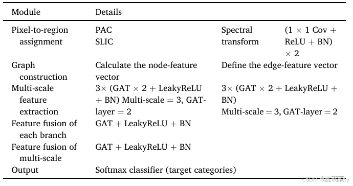
②The architectural details of MRGAT:

③Framework of MRGAT:

④Running times: 10

⑤Training samples per class: 30

2.5.2. Dataset description and processing

①Pavia University, with 103 of 115 bands after processing, 9 classes and size of 610*340:

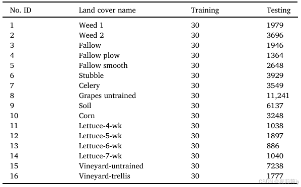
②Salinas, with 204 of 224 bands after removing water vapor absorption bands, 16 categories and size of 512*217:

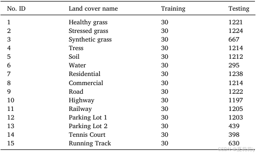
③Houston 2013, with 144 bands, 15 classes, size of 364-1046 nm:

④震撼人心的高光谱仪器，即便不知道是哪里来的，就没有一点版权问题吗？？看作者也没有自己收集：

2.5.3. Classification results

①Performance on Pavia University:

②Performance on Salinas:

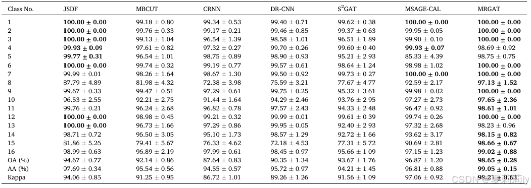
③Performance on Houston 2013:

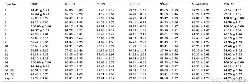
2.5.4. Analysis of the parameter effect

①Ablation of $L$ and $K$ ((a) Pavia University. (b) Salinas. (c) Houston 2013):

②Ablation of $N$ amd $T$ ((a) Pavia University. (b) Salinas. (c) Houston 2013):

2.5.5. The performances with limited labeled samples

①Performance at limited labelled data trained:

2.5.6. Ablation study

①Module ablation:

2.5.7. Training time comparison

①Training time:

2.6. Conclusion

3. Reference

Ding, Y. et al. (2023) Multi-scale receptive fields: Graph attention neural network for hyperspectral image classification, Expert Systems with Applications, 223. doi: Redirecting